
Information theory path: 1. BPSK in AWGN → 2. Shannon capacity (you are here) → 3. Shannon limit on power efficiency · Tool: Shannon–Hartley capacity calculator
In one sentence: the Shannon–Hartley theorem says that a channel of bandwidth $B$ hertz, disturbed by additive white Gaussian noise, can carry at most
$$C = B \log_2\left(1 + \mathrm{SNR}\right) \quad \text{bits/s}$$
with an error rate as small as you like. Below $C$, good coding can make errors vanish. Above $C$, nothing can.
That formula fits on a sticky note, but there’s a lot packed into it. In this article I’ll walk you through what it really promises, how to plug numbers into it without the classic dB mistake, why extra bandwidth stops helping at some point, where the famous $-1.59$ dB comes from, and how far real modulation schemes sit from the limit. There’s Python and Matlab code at the end to reproduce the plots.
What “capacity” actually means: shannon channel capacity
Before 1948, engineers believed that the only way to make a noisy link more reliable was to slow it down. Send each bit more slowly (or repeat it), and errors drop; want zero errors, and the rate drops to zero.
Claude Shannon showed that this intuition is wrong [1]. His noisy channel coding theorem says every channel has a number $C$, its capacity, with two sharp properties:
- If your information rate $R < C$, there exist codes that make the error probability as small as you want, without the rate going to zero.
- If $R > C$, the error probability can’t be driven to zero, no matter how clever the code.
The catch is in the word “exist”. Shannon proved the codes are out there but didn’t hand them to us. Getting close to $C$ takes long codewords (more delay) and heavy decoding (more computation). It took about 45 years, until turbo codes in 1993, for practical codes to come within a dB of the limit. Today’s LDPC and polar codes in 5G NR live in that same neighbourhood.
So capacity isn’t the rate of any particular modem. It’s a ceiling that no modem can beat, and a target that good ones get close to.
The Shannon–Hartley formula
For a channel with bandwidth $B$ Hz, average received signal power $P$ watts, and white Gaussian noise of one-sided power spectral density $N_0$ W/Hz, the noise power in the band is $N_0 B$, and the capacity is [2]:
$$C = B \log_2\left(1 + \frac{P}{N_0 B}\right) \quad \text{bits/s}.$$
The ratio $P/(N_0 B)$ is the signal-to-noise ratio in the band, so the familiar short form is
$$C = B \log_2\left(1 + \mathrm{SNR}\right).$$
Each part of the formula has a plain meaning:
- Bandwidth $B$ sets how many independent symbols per second you can send (roughly $B$ complex symbols per second, by Nyquist).
- $\log_2(1 + \mathrm{SNR})$ is how many bits each of those symbols can carry before the noise blurs neighbouring levels together.
Dividing by $B$ gives the spectral efficiency, the best possible bits per second per hertz:
$$\eta = \frac{C}{B} = \log_2\left(1 + \mathrm{SNR}\right) \quad \text{bits/s/Hz}.$$
A quick note on real and complex channels: for a real baseband channel of bandwidth $B$ with two-sided noise density $N_0/2$, and for a passband radio channel of RF bandwidth $B$ written in complex baseband, you get the same formula. In both cases the noise power in the band is $N_0 B$.
Worked examples (and the dB trap)
The SNR inside the log is a linear power ratio, not decibels. Always convert first:
$$\mathrm{SNR} = 10^{\mathrm{SNR_{dB}}/10}.$$
Telephone line. A voice channel has about $B = 3$ kHz and an SNR of 30 dB, which is $10^{3} = 1000$:
$$C = 3000 \log_2(1 + 1000) \approx 29.9 \text{kbit/s}.$$
That’s why dial-up modems topped out around 33.6 kbit/s: they were already pushing against Shannon. (The later 56k modems went beyond that by avoiding one analog-to-digital conversion, which removes most of the quantization noise and so raises the effective SNR.)
If you forget to convert and plug in 30 instead of 1000, you get $3000 \log_2 31 \approx 14.9$ kbit/s, half the right answer. This is the single most common mistake I see in student assignments.
Wi-Fi channel. $B = 20$ MHz at 25 dB SNR ($\approx 316$):
$$C = 20 \times 10^{6} \log_2(1 + 316.2) \approx 166 \text{Mbit/s}.$$
5G NR carrier. $B = 100$ MHz at 20 dB SNR, per spatial layer:
$$C = 100 \times 10^{6} \log_2(1 + 100) \approx 666 \text{Mbit/s}.$$
Going backwards. You can also ask: what SNR do I need for a given rate? Invert the formula:
$$\mathrm{SNR}_{min} = 2^{C/B} – 1.$$
To push 1 Mbit/s through 200 kHz you need $\eta = 5$ bits/s/Hz, so $\mathrm{SNR} \ge 2^{5} – 1 = 31$, about 14.9 dB.
You can check any of these in the Shannon–Hartley capacity calculator.
Capacity versus SNR: two regimes
Figure 1 plots the spectral efficiency against SNR. The curve has two very different personalities.
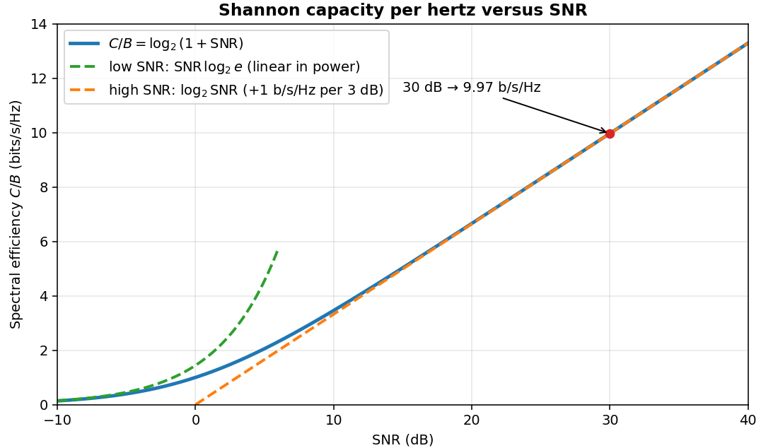
High SNR ($\mathrm{SNR} \gg 1$): the “1 +” hardly matters, so
$$\eta \approx \log_2 \mathrm{SNR} = \frac{\mathrm{SNR_{dB}}}{10 \log_{10} 2} \approx \frac{\mathrm{SNR_{dB}}}{3.01}.$$
Every extra 3 dB buys only one more bit/s/Hz. Doubling your transmit power gives you a small, fixed increment. This is the bandwidth-limited regime, where spectrum is the precious resource.
Low SNR ($\mathrm{SNR} \ll 1$): use $\ln(1 + x) \approx x$:
$$\eta \approx \mathrm{SNR} \cdot \log_2 e \approx 1.44 , \mathrm{SNR}.$$
Now capacity grows linearly with power. Double the power and you double the rate. This is the power-limited regime: deep-space probes, IoT sensors at the cell edge, GPS.
A handy consequence: doubling the bandwidth (at the same power) beats doubling the power whenever the SNR is above 6 dB. Below that, power wins. You can check it yourself: $2\log_2(1 + \mathrm{SNR}/2) > \log_2(1 + 2,\mathrm{SNR})$ only when $\mathrm{SNR} > 4$. Take the 5G example above. Doubling the power (20 → 23 dB) lifts capacity from 666 to 765 Mbit/s. Doubling the bandwidth to 200 MHz (with the same power, so SNR falls to 17 dB) lifts it to 1135 Mbit/s.
Why infinite bandwidth doesn’t give infinite capacity
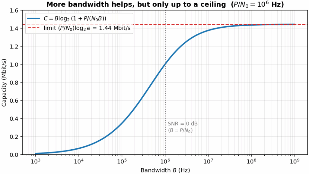
If bandwidth is so valuable, can we just keep adding it? Not quite. Hold the received power $P$ fixed and increase $B$: the noise power $N_0 B$ grows too, so the SNR falls. The two effects balance out, and capacity approaches a finite ceiling:
$$\lim_{B \to \infty} B \log_2\left(1 + \frac{P}{N_0 B}\right) = \frac{P}{N_0} \log_2 e \approx 1.44 \, \frac{P}{N_0} \quad \text{bits/s}.$$
Figure 2 shows this for $P/N_0 = 10^{6}$ Hz. Capacity climbs steeply while the SNR is high, bends over around $B = P/N_0$ (where SNR = 0 dB), and creeps up to 1.44 Mbit/s. Beyond that point, the only way to go faster is more power.
The Shannon limit in terms of Eb/N0: −1.59 dB
Engineers often prefer $E_b/N_0$, the energy per information bit relative to the noise density, because it lets you compare schemes with different rates and bandwidths fairly. The two are related by $P = E_b R$, so
$$\mathrm{SNR} = \frac{E_b}{N_0} \cdot \frac{R}{B}.$$
Operate exactly at capacity ($R = C$, so $R/B = \eta$) and substitute into $\eta = \log_2(1 + \mathrm{SNR})$:
$$2^{\eta} = 1 + \eta \frac{E_b}{N_0} quad \Longrightarrow \quad \frac{E_b}{N_0} = \frac{2^{\eta} – 1}{\eta}.$$
This is the minimum $E_b/N_0$ needed for reliable communication at spectral efficiency $\eta$. At $\eta = 1$ it’s exactly 1 (0 dB). At $\eta = 2$ it’s 1.5 (1.76 dB). And as $\eta \to 0$, meaning we spend unlimited bandwidth on each bit:
$$\lim_{\eta \to 0} \frac{2^{\eta} – 1}{\eta} = \ln 2 \approx 0.693 \quad \Longrightarrow \quad -1.59 \text{dB}.$$
That’s the Shannon limit. No system on an AWGN channel, with any code and any amount of bandwidth, can communicate reliably below $E_b/N_0 = -1.59$ dB. The full story of this limit is in Shannon’s limit on power efficiency.
Figure 3 is the classic chart every comms engineer should know. The blue curve is the boundary. The orange squares show uncoded Gray-coded modulation at a bit error rate of $10^{-5}$.
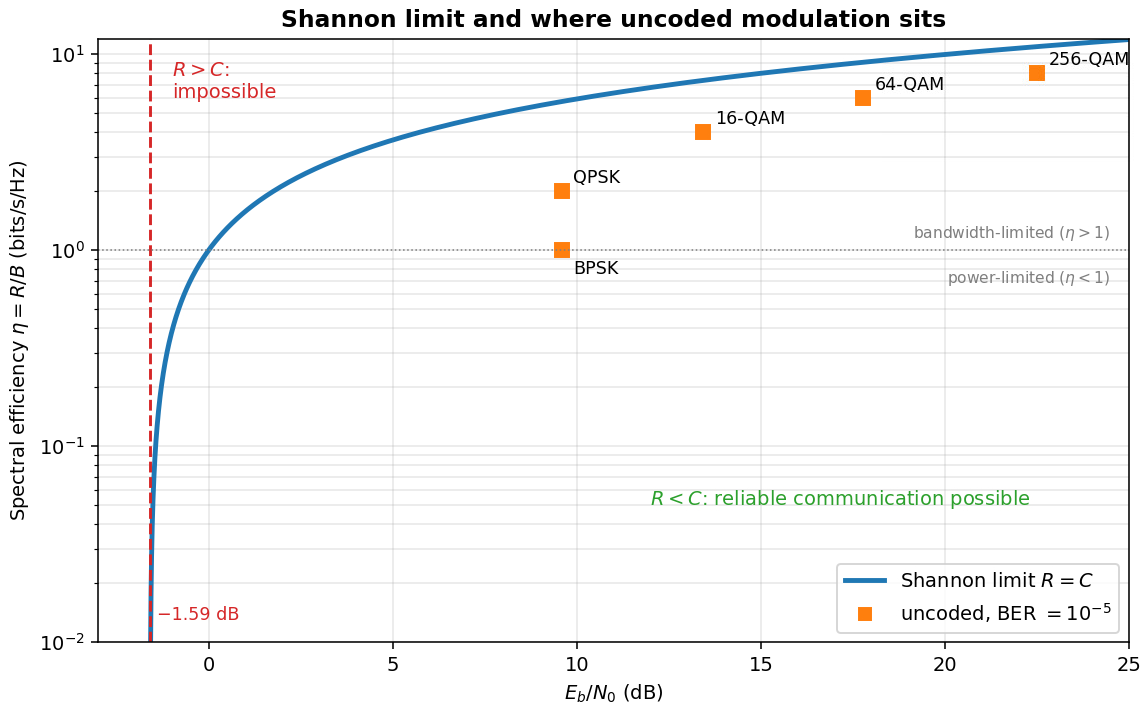
Look at the horizontal distance from each square to the curve:
| Scheme | $\eta$ (bits/s/Hz) | Uncoded $E_b/N_0$ at BER $10^{-5}$ | Shannon limit | Gap |
|---|---|---|---|---|
| BPSK | 1 | 9.6 dB | 0.0 dB | 9.6 dB |
| QPSK | 2 | 9.6 dB | 1.8 dB | 7.8 dB |
| 16-QAM | 4 | 13.4 dB | 5.7 dB | 7.7 dB |
| 64-QAM | 6 | 17.8 dB | 10.2 dB | 7.6 dB |
| 256-QAM | 8 | 22.5 dB | 15.0 dB | 7.5 dB |
Uncoded modulation wastes roughly 7.5 to 10 dB. That gap is the playground of error-correcting codes. A good LDPC code pays a bit of spectral efficiency (the code rate) to win back most of those decibels. You can compute the uncoded points yourself in the BER vs Eb/N0 calculator, and convert between $E_b/N_0$ and SNR with the Eb/N0–SNR converter.
What if the constellation is fixed?
Shannon’s formula assumes the transmitted symbols can take any value, with a Gaussian distribution. Real systems use a fixed alphabet such as QPSK or 64-QAM. With $M$ points, you obviously can’t carry more than $\log_2 M$ bits per symbol, however clean the channel.
Figure 4 shows the achievable rate (the mutual information) of each constellation with equally likely points, computed by Monte Carlo simulation.
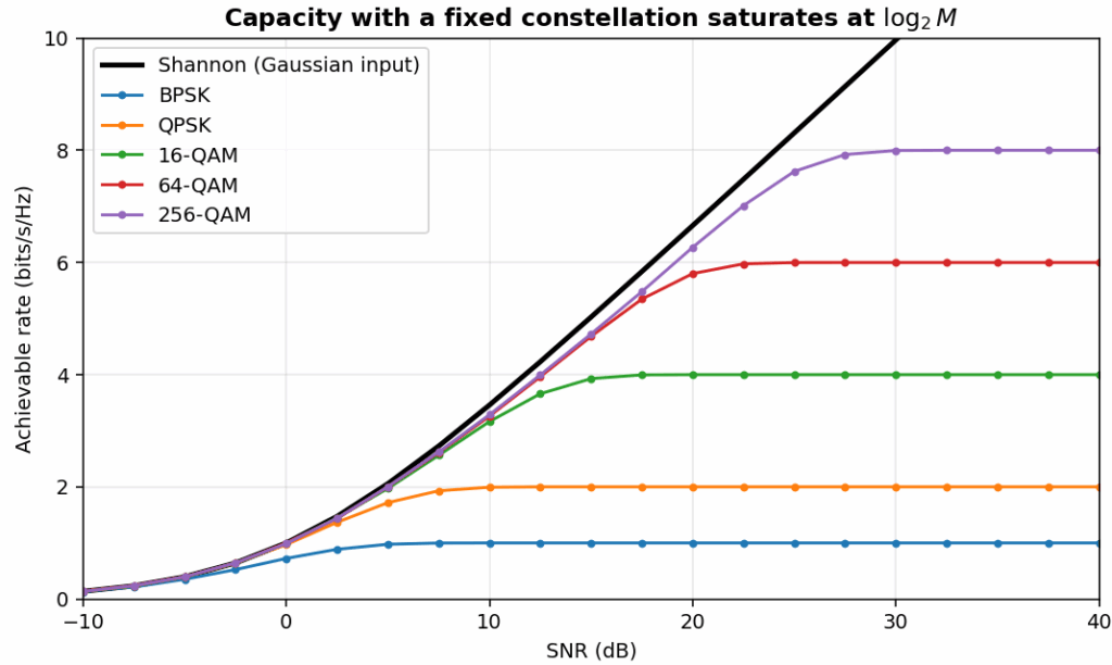
Three lessons drop out of this plot:
- At low SNR all constellations hug the Shannon curve. There, QPSK is as good as anything.
- Each curve flattens at $\log_2 M$. That’s why systems switch to bigger constellations as SNR improves. In 5G NR, link adaptation picks among QPSK, 16-QAM, 64-QAM, 256-QAM and 1024-QAM plus a code rate, based on the reported channel quality.
- Even 256-QAM sits slightly below the Shannon curve before it saturates. At 5 bits/s/Hz it needs about 1 dB more SNR than Shannon, and the gap grows toward a theoretical 1.53 dB at high rates. Uniformly spaced, equally likely points aren’t Gaussian. Techniques like probabilistic constellation shaping close part of this gap.
Shannon versus Nyquist
Students often ask how this relates to the Nyquist formula $C = 2B \log_2 M$ (for a real channel with $M$ signal levels). Nyquist’s formula is for a noiseless channel. It says how fast you can signal, but it puts no limit on $M$: with no noise, you could use a million levels.
Shannon’s formula adds the noise. Equating the two for a real channel gives the largest number of levels that noise allows you to tell apart reliably:
$$M \approx \sqrt{1 + \mathrm{SNR}}.$$
At 30 dB, that’s about 32 levels per real dimension. Ralph Hartley had already linked rate to the number of distinguishable levels in 1928 [3], which is why the theorem carries both names.
A little history
The ideas didn’t appear from nowhere. In 1903, W. M. Miner patented time-division multiplexing on telephone lines using sampling [4]. In 1936, Edwin Armstrong showed that wideband FM could improve SNR at the cost of extra bandwidth [5], a concrete case of trading bandwidth for SNR. In 1937, Alec Reeves invented pulse code modulation (patented in France in 1938 and in the US in 1942 [6]), which showed that quantized samples could be sent almost error-free if the SNR was high enough. Shannon tied these threads together in 1948 [1] and gave the clean, sampling-theorem-based derivation for the band-limited Gaussian channel a year later [2]. For a textbook proof, see Cover and Thomas [7].
Python code
This script reproduces the worked examples, prints the Shannon limit, and draws Figure 1.
import numpy as np
import matplotlib.pyplot as plt

def capacity(B, snr_db):
    """Shannon-Hartley capacity in bits/s. SNR given in dB."""
    snr = 10**(np.asarray(snr_db) / 10)   # dB -> linear, never skip this
    return B * np.log2(1 + snr)

print(f"Telephone 3 kHz, 30 dB : {capacity(3e3, 30)/1e3:6.1f} kbit/s")
print(f"Wi-Fi 20 MHz, 25 dB    : {capacity(20e6, 25)/1e6:6.1f} Mbit/s")
print(f"5G NR 100 MHz, 20 dB   : {capacity(100e6, 20)/1e6:6.1f} Mbit/s")
print(f"SNR for 5 bit/s/Hz     : {10*np.log10(2**5 - 1):6.2f} dB")
print(f"Shannon limit Eb/N0    : {10*np.log10(np.log(2)):6.2f} dB")

P_N0 = 1e6                            # P/N0 in Hz
for B in [1e5, 1e6, 1e7, 1e8]:
    C = B * np.log2(1 + P_N0 / B)
    print(f"B = {B:8.0e} Hz -> C = {C/1e6:.3f} Mbit/s")
print(f"Wideband limit         : {P_N0*np.log2(np.e)/1e6:.3f} Mbit/s")

snr_db = np.linspace(-10, 40, 501)
plt.plot(snr_db, capacity(1, snr_db), lw=2, label='log2(1 + SNR)')
plt.plot(snr_db, np.log2(10**(snr_db/10)), '--', label='high-SNR approx.')
plt.xlabel('SNR (dB)')
plt.ylabel('Spectral efficiency (bits/s/Hz)')
plt.ylim(0, 14)
plt.grid(alpha=0.3)
plt.legend()
plt.show()Output:
Telephone 3 kHz, 30 dB :   29.9 kbit/s
Wi-Fi 20 MHz, 25 dB    :  166.2 Mbit/s
5G NR 100 MHz, 20 dB   :  665.8 Mbit/s
SNR for 5 bit/s/Hz     :  14.91 dB
Shannon limit Eb/N0    :  -1.59 dB
B =    1e+05 Hz -> C = 0.346 Mbit/s
B =    1e+06 Hz -> C = 1.000 Mbit/s
B =    1e+07 Hz -> C = 1.375 Mbit/s
B =    1e+08 Hz -> C = 1.436 Mbit/s
Wideband limit         : 1.443 Mbit/s
Matlab code
The same calculation in Matlab, plus the Shannon-limit curve of Figure 3:
capacity = @(B, snrdB) B .* log2(1 + 10.^(snrdB/10));   % bits/s

Cphone = capacity(3e3, 30)/1e3      % 29.9 kbit/s
Cwifi  = capacity(20e6, 25)/1e6     % 166.2 Mbit/s
C5g    = capacity(100e6, 20)/1e6    % 665.8 Mbit/s

limit_dB = 10*log10(log(2))         % -1.59 dB

eta     = logspace(-2, log10(12), 400);        % bits/s/Hz
ebn0_dB = 10*log10((2.^eta - 1)./eta);         % Eb/N0 needed at R = C
semilogy(ebn0_dB, eta, 'LineWidth', 2); hold on;
xline(limit_dB, '--r', '-1.59 dB');
xlabel('E_b/N_0 (dB)'); ylabel('Spectral efficiency (bits/s/Hz)');
title('Shannon limit'); grid on;Questions readers often ask
Does the capacity include the error-correction bits, or only the information? Only the information. $C$ is the maximum rate of useful data. If a link has $C = 1000$ bit/s and you use a rate-1/2 code, the coded bit rate on the wire can be 2000 bit/s, but the information rate must stay below 1000 bit/s.
If I transmit below capacity, do I still need error-correcting codes? Yes. Shannon’s theorem says low error rates are achievable below $C$, and the way you achieve them is coding. An uncoded system running at a rate well below $C$ can still have a poor BER, as the gaps in Figure 3 show.
What are “capacity-approaching codes”? Codes whose required $E_b/N_0$ at a target error rate comes within a fraction of a dB of the Shannon limit for their spectral efficiency. Turbo codes (3G/4G), LDPC codes (Wi-Fi, DVB-S2, 5G NR data channels) and polar codes (5G NR control channels) are the main examples.
If I send a single pure sine wave, is the capacity zero? A pure, unmodulated carrier occupies zero bandwidth and carries no information, so yes, $C = 0$ is the right answer. The moment you modulate it (even with on-off keying), it occupies non-zero bandwidth and the formula applies to that bandwidth.
The −1.59 dB limit assumes infinite bandwidth. How can it be a limit for a band-limited system? It’s a limit on power efficiency, not bandwidth. With finite bandwidth you need more than −1.59 dB, given by $(2^{\eta} – 1)/\eta$. Infinite bandwidth is the best case, and even then you can’t go below −1.59 dB.
How can I increase the capacity of a channel? In the AWGN formula there are only two knobs: bandwidth and SNR. Raise the SNR with more transmit power, better antennas or a quieter receiver. Raise bandwidth with more spectrum or carrier aggregation. With multiple antennas, MIMO opens a third knob: parallel spatial streams. See Capacity of a MIMO system over fading channels.
Does the formula hold for fading channels? Not directly. It’s for AWGN with a fixed SNR. Over fading, you average the formula over the fading distribution (ergodic capacity) or ask for the rate that’s supported with a given probability (outage capacity).
Keep learning
- Shannon–Hartley channel capacity calculator: plug in bandwidth and SNR
- Shannon’s limit on power efficiency: the −1.59 dB story in depth
- BPSK modulation and demodulation: an uncoded point on Figure 3, simulated
- Capacity of a MIMO system over fading channels
- BER vs Eb/N0 calculator and Eb/N0, Es/N0 and SNR converter
Want the complete lab notebooks? The Digital Modulations using Python ebook gives you the full simulation code, exercises, and constellation and BER chapters. Compare all books.
References
- C. E. Shannon, “A Mathematical Theory of Communication,” Bell System Technical Journal, vol. 27, pp. 379–423 and 623–656, July and October 1948. doi:10.1002/j.1538-7305.1948.tb01338.x
- C. E. Shannon, “Communication in the Presence of Noise,” Proc. IRE, vol. 37, no. 1, pp. 10–21, January 1949. doi:10.1109/JRPROC.1949.232969
- R. V. L. Hartley, “Transmission of Information,” Bell System Technical Journal, vol. 7, no. 3, pp. 535–563, July 1928. doi:10.1002/j.1538-7305.1928.tb01236.x
- W. M. Miner, “Multiplex Telephony,” US Patent 745,734, December 1903. Google Patents
- E. H. Armstrong, “A Method of Reducing Disturbances in Radio Signaling by a System of Frequency Modulation,” Proc. IRE, vol. 24, no. 5, pp. 689–740, May 1936. doi:10.1109/JRPROC.1936.227383
- A. H. Reeves, “Electric Signaling System,” US Patent 2,272,070, February 1942. Google Patents
- T. M. Cover and J. A. Thomas, Elements of Information Theory, 2nd ed., Wiley, 2006, Chapter 9.
Dear Sir,
If I use only one Sine wave (say f=10Hz), then is the bandwidth zero (since fH = 10Hz and fL = 10Hz)? Then is the capacity zero? Say modulation is on-off keying to communicate 1 bit data.
When can the capacity be zero?
Thank you.
Two scenarios here,
If the system is a low pass system , the bandwidth is 10Hz. You can apply Shannon capacity equation and find the capacity for the given SNR.
If the system is a bandpass system, since fH=FL=10Hz, it is assumed to be same as some carrier frequency fc=10Hz. Thus the bandwidth is zero (nothing around the carrier frequency) and if you apply the shannon capacity equation for AWGN, C is zero in this case. This calculation of capacity seems absurd, as we know that we not sending any information (just a carrier here and no information ) and therefore capacity is zero. By doing this calculation we are not achieving anything.
Hi
1)We have to use error control coding to reduce BER in the noisy channel even if we send the data much below the capacity of the channel… am i right ?
2)If i say the channel has the capacity 1000 bits/sec ( as per Shannon – Hartley Equation)
this 1000 bit/s is ( information + error control data) OR information alone ( excluding error control data)..???
3)can you elaborate on capacity reaching codes ? which capacity they are trying to reach ?
How the “unconstrained Shannon power efficiency Limit” is a limit for band limited system when you assumed B = infinite while determining this value?
The term “limit” is used for power efficiency (not for bandwidth).
This tells us , now matter how much bandwidth we have (B-> infinity), the transmission power should always be more than the Shannon power efficiency limit in terms of Eb/N0 (-1.59 dB)
Hello Sir, i’m a master student and i have a problem in one of my codes, can i please have your email address to contact with you. it will not take much of your time.
Nice blog, throughout and clear!
How channel capacity can be increased numerically using the definition of information?