Chi square distribution – demystified

A random variable is always associated with a probability distribution. When the random variable undergoes mathematical transformation the underlying probability distribution no longer remains the same. Consider a random variable $latex Z $ whose probability distribution function (PDF) is a standard normal distribution ($latex \mu=0 $ and $latex \sigma^2=1 $). Now, if the random variable is squared (a mathematical transformation), then the PDF of $latex Z^2 $ is no longer a standard normal distribution. The new transformed distribution is called Chi square Distribution with $latex 1 $ degree of freedom. The PDF of $latex Z $ and $latex Z^2 $ are plotted in Figure 1.

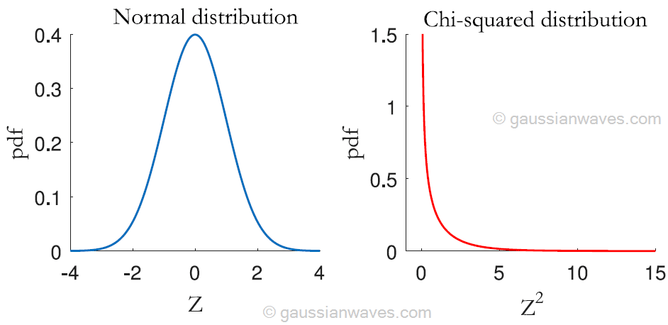
The mean of the random variable $latex Z $ is $latex E(Z) = 0 $ and for the transformed variable Z², the mean is given by $latex E(Z^2)=1 $. Similarly, the variance of the random variable $latex Z $ is $latex \sigma^2_Z=1 $, whereas the variance of the transformed random variable $latex Z^2 $ is $latex \sigma^2_{Z^2}=2 $. In addition to the mean and variance, the shape of the distribution is also changed. The distribution of the transformed variable $latex Z^2 $ is no longer symmetric. In fact, the distribution is skewed to one side. Also the random variable $latex Z^2 $ can take only positive values whereas the random variable $latex Z $ can take negative values too (note the x-axis in the plots above).

Since the new transformation is based on only one parameter ($latex Z $), the degree of freedom for this transformation is $latex 1 $. Therefore, the transformed random variable $latex Z^2 $ follows – “Chi-square distribution with $latex 1 $ degree of freedom”.
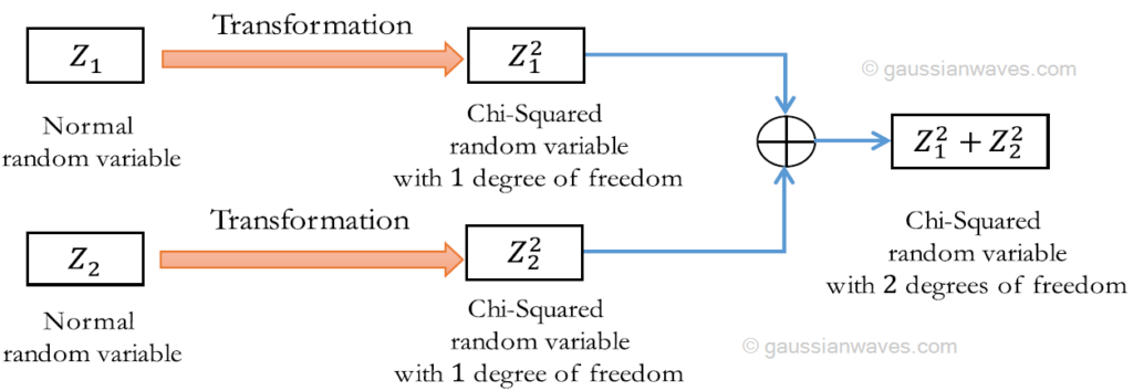
Suppose, if $latex Z_1,Z_2,\cdots,Z_k $ are independent random variables that follows standard normal distribution($latex \mu=0 $ and $latex \sigma^2=1 $), then the transformation,

$latex \chi_k^2 = Z_1^2 + Z_2^2+ \cdots+Z_k^2 $

is a Chi square distribution with k degrees of freedom. The following figure illustrates how the definition of the Chi square distribution as a transformation of normal distribution for $latex 1 $ degree of freedom and $latex 2 $ degrees of freedom. In the same manner, the transformation can be extended to $latex k $ degrees of freedom.

The above equation is derived from $latex k $ random variables that follow standard normal distribution. For a standard normal distribution, the mean $latex \mu=0 $. Therefore, the transformation $latex \chi_k^2 $ is called central Chi-square distribution. If, the underlying $latex k $ random variables follow normal distribution with non-zero mean, then the transformation $latex \chi_k^2 $ is called non-central Chi-square distribution [2] . In channel modeling, the central Chi-squared distribution is related to Rayleigh Fading scenario and the non-central Chi-square distribution is related to Rician Fading scenario.

Mathematically, the PDF of the central Chi-squared distribution with $latex k $ degrees of freedom is given by

$latex f_{\chi_k^2 }(x)= \frac{1}{2^{\frac{k}{2}}\Gamma \left(\frac{k}{2}\right )}x^{\frac{k}{2}-1}e^{-\frac{x}{2}} $

The mean and variance of the central Chi-squared distributed random variable is given by

$latex \mu = E\left[\chi_k^2\right] = k $

$latex \sigma^2 = var\left[\chi_k^2\right] = 2k $

Relation to Rayleigh distribution

The connection between Chi square distribution and the Rayleigh distribution can be established as follows

1. If a random variable $latex R $ has standard Rayleigh distribution, then the transformation $latex R^2 $ follows chi-square distribution with $latex 2 $ degrees of freedom.
2. If a random variable $latex C $ has the chi-square distribution with $latex 2 $ degrees of freedom, then the transformation $latex \sqrt{C} $ has standard Rayleigh distribution.

Applications:

Chi-square distribution is used in hypothesis testing (to compare the observed data with expected data that follows a specific hypothesis) and in estimating variances of a parameter.

Matlab Simulation:

Check this book for full Matlab code.
Wireless Communication Systems using Matlab – by Mathuranathan Viswanathan

Python Code

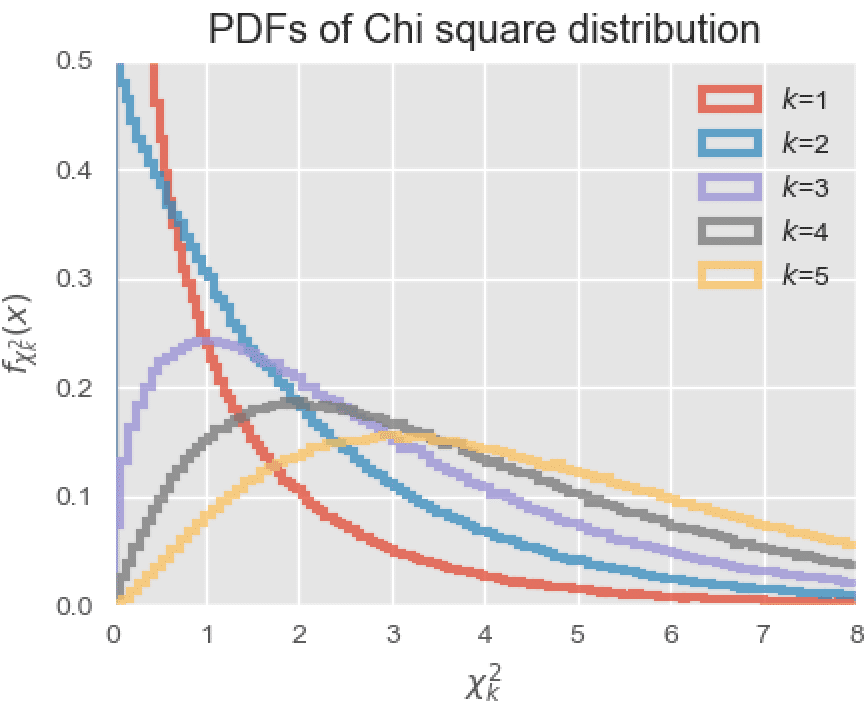
Python numpy package has a chisquare() generator, which can be used in a straightforward manner to obtain the Chi square distributed sequences.

#---------Chi square distribution gaussianwaves.com-----
import numpy as np
import matplotlib.pyplot as plt
#%matplotlib inline
plt.style.use('ggplot')

ks=np.arange(start=1,stop=6,step=1) #degrees of freedoms to simulate
nSamp=1000000 #number of samples to generate

fig, ax = plt.subplots(ncols=1, nrows=1, constrained_layout=True)

for i,k in enumerate(ks):
    #Generate central Chi-square distributed random numbers
    X = np.random.chisquare(df=k, size = nSamp)
    ax.hist(X,bins=500,density=True,label=r'$k$={}'.format(k), \
    histtype='step',alpha=0.75, linewidth=3)

ax.set_xlim(left=0,right=8);ax.set_ylim(bottom=0,top=0.5);ax.legend();
ax.set_title('PDFs of Chi square distribution');
ax.set_xlabel(r'$\chi_k^2$');ax.set_ylabel(r'$f_{\chi_k^2}(x)$');
plt.show()

For further reading

[1] Ernie Croot, “Notes on Chi-squared distribution”, Georgia institute of technology, School of mathematics, Oct 2005.↗