
Spreading codes path:
m-sequences → Gold codes → CDMA codes
In one sentence: An m-sequence is the longest period binary sequence from an n-stage LFSR ($latex 2^n-1$), with near-ideal two-valued periodic autocorrelation.
Key focus: Model and simulate m-sequence generator using Galois linear feedback shift registers (LFSR) that implement linear recursion. Plot correlation properties.
Maximum-length sequences (also called as m-sequences or pseudo random (PN) sequences) are constructed based on Galois field theory which is an extensive topic in itself. A detailed treatment on the subject of Galois field theory can be found in references [1] and [2].
Maximum length sequences are generated using linear feedback shift registers (LFSR) structures that implement linear recursion. There are two types of LFSR structures available for implementation – 1) Galois LFSR and 2) Fibonacci LFSR. The Galois LFSR structure is a high speed implementation structure, since it has less clock to clock delay path compared to its Fibonacci equivalent. What follows in this discussion is the implementation of an m-sequence generator based on Galois LFSR architecture (Figure 1).
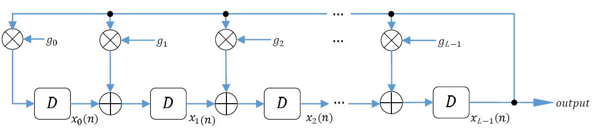
The basic Galois LFSR architecture for an $latex L^{th}$-order generating polynomial in $latex GF(2)$ is given in Figure 1. The integer value $latex L$ denotes the number of delay elements in the LFSR architecture and $latex g_0,g_1,…,g_{L}$ represent the coefficients of the generator polynomial. The generator polynomial of the given LFSR is

where, $latex g_0,g_1,…,g_{L-1} \in GF(2)$, i.e, they take only binary values. The first and last coefficients are usually unity: $latex g_0=g_{L}=1$.
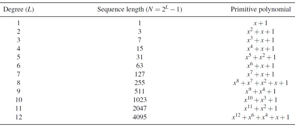
For generating an m-sequence, the characteristic polynomial that dictates the feedback coefficients, should be a primitive polynomial. Table 1 lists some of the primitive polynomials of degree upto $latex L=12$. More comprehensive tables of primitive polynomials can be found in reference [3].
For implementation in Matlab, the LFSR structure can be coded in a straightforward manner that involves at least two for loops. If we could exploit the linear recursion property of LFSR and its equivalent matrix model, the LFSR can be implemented using only one for loop as shown in the Matlab function given in the book (click here). The function implements the LFSR structure Figure 1 by using the following equivalent matrix equation:
$latex \mathbf{x}(n+1) = \mathbf{A} \mathbf{x}(n), \quad n >=0 \quad (2) &s=2$
with the initial state of the shift registers represented by the vector $latex \mathbf{x}(0)$, and $latex \mathbf{x}(n)$ is an $latex L$ dimensional vector given by
$latex \mathbf{A}= \begin{bmatrix} \mathbf{x}_0(n) & \mathbf{x}_1(n) & \cdots & \mathbf{x}_{L-1}(n)\end{bmatrix}^T \quad \quad(3) &s=2$
The matrix $latex \mathbf{A}$ is of dimension $latex L \times L $, given by
$latex \mathbf{A}= \begin{bmatrix} 0 & 0 & 0 & \cdots & 0 & g_0\\ 1 & 0 & 0 & \cdots & 0 & g_1 \\ 0 & 1 & 0 & \cdots & 0 & g_2\\ 0 & 0 & 1 & \cdots & 0 & g_3\\ \vdots & \vdots & \vdots & \ddots & \vdots & \vdots \\ 0 & 0 & 0 & \cdots & 1 & g_{L-1} \end{bmatrix} \quad\quad (4) &s=2$
Correlation properties of m-sequences are demonstrated here. It uses the sequence_correlation function defined in section 12.2.1 in the book (click here).
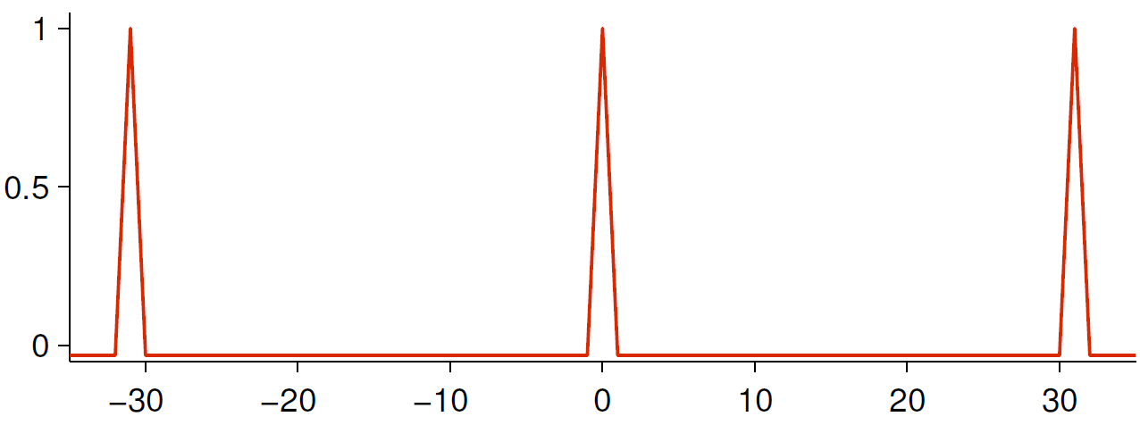
Let’s generate an m-sequence of period $latex N=31$ using the $latex 5^{th}$ order characteristic polynomial $latex g(x)=x^5+x^2+1$. The coefficients of the characteristic polynomial is $latex G=[g_5,g_4,g_3,g_2,g_1,g_0]=[1,0,0,1,0,0]$ and let’s start the generator with initial seed $latex X_0=[0,0,0,0,1]$. Typically, the autocorrelation function of m-sequences are two valued. The normalized autocorrelation of an m-sequence of length $latex N$, takes two values $latex [1,-1/N]$. This is demonstrated in Figure 2. We observe that that autocorrelation of m-sequence carries some similarities with that of a random sequence. If the length of the m-sequence is increased, the out-of-peak correlation $latex -1/N$ reduces further and thereby the peaks become more distinct. This property makes the m-sequences suitable for synchronization and in the detection of information in single-user Direct Sequence Spread Spectrum systems.
To demonstrate cross-correlation properties of two different m-sequences, consider two different primitive polynomials $latex g_1(x)=x^5+x^4+x^2+x+1$ and $latex g_2(x)=x^5+x^4+x^3+x+1$ that could generate two different m-sequences of length $latex N=31$. The normalized cross-correlation of the aforementioned m-sequences, shown in Figure 3, is given by the Matlab script given in the book (click here).

The cross-correlation plot contains high peaks at certain lags (as high as $latex 35\%$) and hence the m-sequences causes multiple access interference↗ (MAI), leading to severe performance degradation. Hence, the m-sequences are not suitable for orthogonalization of users in multi-user spread spectrum systems like CDMA.
Continue reading on generation of Gold codes using preferred pair m-sequences…
References
[1] D. V. Sarwate and M. B. Pursley, Crosscorrelation properties of pseudorandom and related sequences, Proc. IEEE, vol. 68, no. 5, pp. 593–619, May 1980.↗
[2] S. W. Golomb, Shift-register sequences and spread-spectrum communications, Proceedings of IEEE 3rd International Symposium on Spread Spectrum Techniques and Applications (ISSSTA’94), Oulu, Finland, 1994, pp. 14-15 vol.1.↗
[3] R. L. Peterson, R. E. Ziemer, and D. E. Borth, Introduction to Spread Spectrum Communications, Prentice Hall, Inc., 1995.↗
FAQ
Why must an LFSR use a primitive polynomial to generate an m-sequence? Only a primitive feedback polynomial over GF(2) makes the shift-register state cycle through all $latex 2^n-1$ nonzero states before repeating. Non-primitive polynomials produce shorter periods and lose the famous two-level autocorrelation.
What does the periodic autocorrelation of an m-sequence look like? With the usual $latex \pm 1$ mapping, the periodic autocorrelation peaks at $latex N=2^n-1$ for lag 0 and equals $latex -1$ at all other lags. That thumbtack shape is why m-sequences are prized for spreading and channel sounding.
What is the natural next code family after m-sequences? Preferred pairs of m-sequences are XOR-combined to build Gold codes, which give a large family with bounded cross-correlation for multi-user CDMA/GNSS.