
OFDM study path — 5 lessons (same on every page in this series)
1. Introduction → 2. Orthogonality (you are here) → 3. IFFT modem → 4. Cyclic prefix → 5. BER in AWGN
In one sentence: Complex tones at integer multiples of $latex 1/T$ are orthogonal on $latex [0,T]$; OFDM places data on those tones so a DFT separates them without ICI when the CP covers delay spread.
Lesson 2 of 5. You already know what OFDM is from the introduction. Here we prove the property that puts the “O” in OFDM. Next you will build the modem with an IFFT.
OFDM, known as Orthogonal Frequency Division Multiplexing, is a digital modulation technique that divides a wideband signal into several narrowband signals. By doing so, it elongates the symbol duration of each narrowband signal compared to the original wideband signal, effectively minimizing the impact of time dispersion caused by multipath delay spread.
OFDM is categorized as a form of multicarrier modulation (MCM), where multiple user symbols are transmitted simultaneously through distinct subcarriers having overlapping frequency bands, ensuring they remain orthogonal to each other.
OFDM implements the same number of channels as the traditional Frequency Division Multiplexing (FDM). Since the channels (subcarriers) are arranged in overlapping manner, OFDM significantly reduces the bandwidth requirement.
OFDM equation
Consider an OFDM system that transmits a user symbol stream $latex s_i$ (rate $latex R_u$) over a set of $latex N$ subcarriers. Therefore, the symbol rate of each subcarrier is $latex R_s = \frac{R_u}{N}$ and the symbol duration is $latex T_s = \frac{N}{R_u}$.
The incoming symbol stream is split into $latex N$ symbols streams and each of the symbol stream is multiplied by a function $latex \Phi_k$ taken from a family of orthonormal functions $latex \Phi_k, k \in \left\{0,1, \cdots, N-1 \right\}$
In OFDM, these orthogonormal functions are complex exponentials
\[\Phi_k (t) = \begin{cases} e^{j 2 \pi f_k t}, & \quad for \; t \in \left[ 0, T_s\right] \\ 0, & \quad otherwise \end{cases} \quad \quad \quad (1) \]For simplicity lets assume BPSK modulation for the user symbol $latex s_i \in \left\{-1,1 \right\}$ and $latex g_i$ is the individual gain of each subchannels. The OFDM symbol is formed by multiplexing the symbols on each subchannels and combining them.
\[S (t) =\frac{1}{N} \sum_{k=0}^{N-1} s_k \cdot g_k \cdot \Phi_k(t) \quad \quad \quad (2)\]The individual subcarriers are
\[s_n (t) = s_k \cdot g_k \cdot e^{j 2 \pi f_k t} \quad \quad \quad (3)\]For a consecutive stream of input symbols $latex m = 0,1, \cdots$ the OFDM equation is given by
\[S(t) = \sum_{m = 0 }^{ \infty} \left[\frac{1}{N} \sum_{k=0}^{N-1} s_{k,m} \cdot g_{k,m} \cdot \Phi_{k}(t – m T_s) \right] \quad \quad \quad (4)\]With $latex g_{k,m} = 1$, the OFDM equation is given by
\[S(t) = \sum_{m = 0 }^{ \infty} \left[\frac{1}{N} \sum_{k=0}^{N-1} s_{k,m} \cdot e^{j 2 \pi f_k \left(t – m T_s \right)} \right] \quad \quad \quad (5)\]Orthogonality
The functions $latex \Phi$ by which the symbols on the subcarriers are multiplied are orthonormal over the symbol period $latex T_s$. That is
\[ \left< \Phi_p (t), \Phi_q (t) \right> = \frac{1}{T_s} \int_{0}^{Ts} \Phi_p (t) \cdot \Phi^*_q (t) dt = \delta_{p,q} \quad \quad \quad (6) \]where, $latex \delta_{p,q}$ is the Kronecker delta given by
\[\delta_{p,q} = \begin{cases} 1, & \quad p=q \\ 0, & \quad otherwise \end{cases} \]The right hand side of equation (5) will be equal to 0 (satisfying orthogonality) if and only if $latex 2 \pi \left(f_p−f_q \right)T_s=2 \pi k$ where $latex k$ is a non-zero integer. This implies that the distance between the two subcarriers, for them to be orthogonal, must be
\[\Delta f = f_p – f_q = \frac{k}{T_s} \quad \quad (7)\]Hence, the smallest distance between two subcarriers, for them to be orthogonal, must be
\[ \Delta f = \frac{1}{T_s} \quad \quad (8)\]This implies that each subcarrier frequency experiences $latex k$ additional full cycles per symbol period compared to the previous carrier. For example, in Figure 1 that plots the real and imaginary parts of three OFDM subcarriers (with $latex k=1$), each successive subcarrier contain additional full cycle per symbol period compared to the previous carrier.

With $latex N$ subcarriers, the total bandwidth occupied by one OFDM symbol will be $latex B \approx N \cdot \Delta f \; (Hz)$

Benefits of orthogonality
Orthogonality ensures that each subcarrier’s frequency is precisely spaced and aligned with the others. This property prevents interference between subcarriers, even in a multipath channel, which greatly improves the system’s robustness against fading and other channel impairments.
The orthogonality property allows subcarriers to be placed close together without causing mutual interference. As a result, OFDM can efficiently utilize the available spectrum, enabling high data rates and maximizing spectral efficiency, making it ideal for high-speed data transmission in wireless communication systems.
FAQ
What is the recommended reading order? Follow the five-lesson path at the top of every page: Introduction → Orthogonality → IFFT modem → Cyclic prefix → BER in AWGN.
What spacing makes two tones orthogonal? Over a block of length $latex T$, spacing must be an integer multiple of $latex 1/T$. The discrete DFT realises exactly that set of bins.
Where does the IFFT fit? The IDFT/IFFT is how the transmitter synthesises those orthogonal tones in one shot — that is lesson 3.
Similar articles
- 1. Introduction to OFDM
- 2. Why OFDM subcarriers are orthogonal
- 3. OFDM with the IFFT (modem)
- 4. Cyclic prefix in OFDM
- 5. OFDM BER simulation in AWGN
- Tool: OFDM CP overhead calculator
- Tool: Eb/N0 ↔ SNR converter
Reference
Numerical check: discrete orthogonality (DFT view)
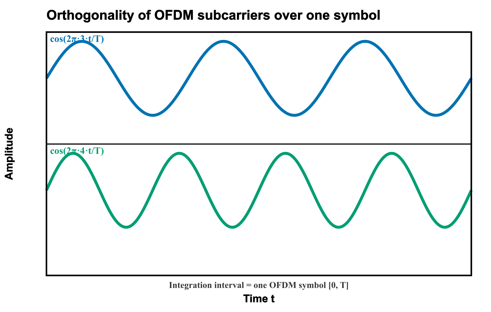
In discrete time with $latex N$ subcarriers, the IDFT tones $latex e^{j 2\pi kn / N}$ are exactly orthogonal over $latex n=0,\ldots,N-1$. That is why the receiver FFT diagonalizes a circular channel (enabled by the cyclic prefix).
import numpy as np

N = 64
n = np.arange(N)
# columns = subcarriers
F = np.exp(1j * 2 * np.pi * np.outer(n, np.arange(N)) / N) / np.sqrt(N)
G = F.conj().T @ F                 # should be ~ I
err = np.max(np.abs(G - np.eye(N)))
print('max off-orthogonality error:', err)

# time-limited mismatch (spectral leakage analogue): use N-1 samples
F_bad = F[:N-1, :]
G_bad = F_bad.conj().T @ F_bad
print('error if one sample missing:', np.max(np.abs(G_bad - np.diag(np.diag(G_bad)))))
If the channel is longer than the CP, circularity breaks and subcarriers leak into each other (ICI). Continue with the CP hands-on demo.