Eb/N0, Es/N0 and SNR — conversions for BER simulations

Introduction: Bit-error-rate theory is almost always written against $latex E_b/N_0$, but your simulator adds noise against a symbol energy $latex E_s$ (and a sampling-rate convention). This article derives the exact conversions among $latex E_b/N_0$, $latex E_s/N_0$, and SNR, then shows how to generate complex baseband AWGN so Monte Carlo curves overlay the textbook formula.

If your simulated BER curve sits neatly below theory, or looks “too good” by a few dB, the first place to look is not the demodulator: it is the noise variance. Mixing up $latex E_b$ and $latex E_s$, forgetting the factor of two between real and complex noise, or ignoring oversampling are the classic mistakes.

1. What $latex E_b$, $latex E_s$, and $latex N_0$ actually mean

Start from continuous-time complex baseband. A digital transmitter emits a sequence of symbols $latex \{s[m]\}$ through a pulse $latex p(t)$ of symbol period $latex T$. The average energy carried by one modulation symbol (after the pulse is normalized appropriately) is $latex E_s$. If each symbol conveys $latex k=\log_2 M$ information bits — for example $latex k=1$ for BPSK, $latex k=2$ for QPSK, $latex k=4$ for 16-QAM — then the average energy per information bit is

$latex E_b = E_s / k$.

Additive white Gaussian noise is characterized by a one-sided power spectral density $latex N_0$ (watts per hertz). In the equivalent complex baseband model the noise is circularly symmetric complex Gaussian with two-sided PSD $latex N_0$ total for the complex envelope (that is, $latex N_0/2$ in each of the in-phase and quadrature dimensions). The dimensionless ratios

$latex \displaystyle \gamma_b = \frac{E_b}{N_0}, \qquad \gamma_s = \frac{E_s}{N_0}$

are the fundamental SNRs of digital communications. Almost every closed-form AWGN BER or SER formula in a textbook is written in terms of $latex \gamma_b$ or $latex \gamma_s$.

The conversion that every simulator needs

Because $latex E_s = k E_b$, the two ratios differ only by the bits-per-symbol factor:

$latex \displaystyle \frac{E_s}{N_0} = k\,\frac{E_b}{N_0}$.

In decibels this becomes a simple offset:

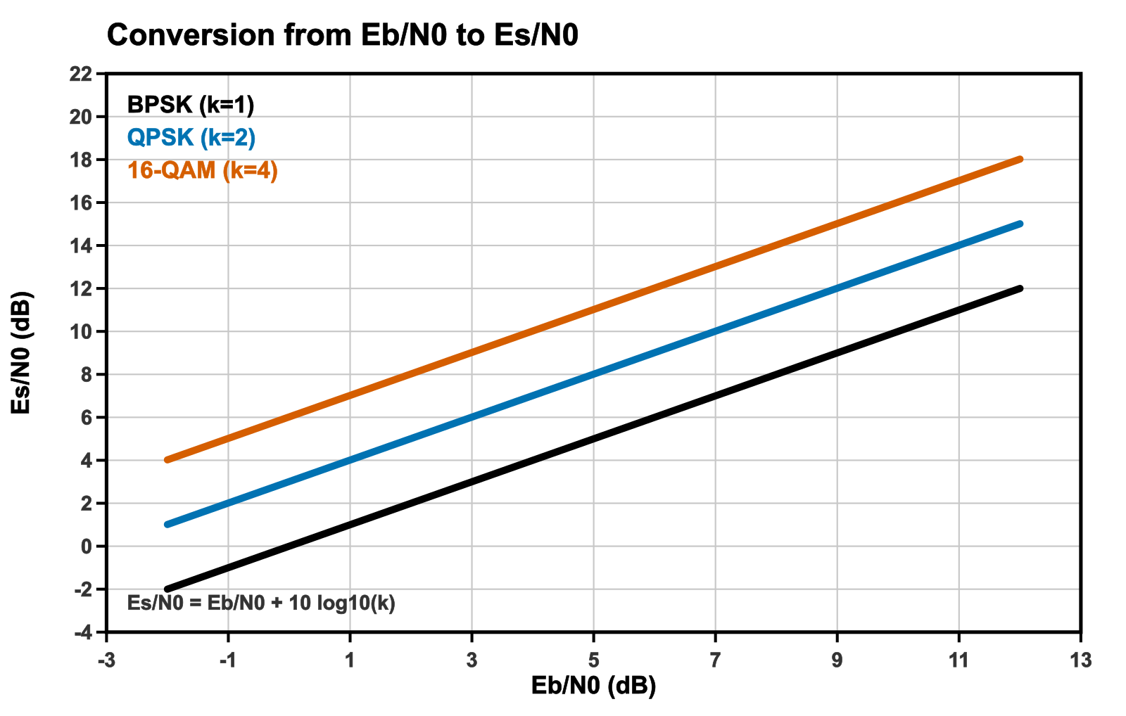
$latex \displaystyle \left.\frac{E_s}{N_0}\right|_{\mathrm{dB}} = \left.\frac{E_b}{N_0}\right|_{\mathrm{dB}} + 10\log_{10} k$.

Numerically: QPSK ($latex k=2$) sits $latex 10\log_{10}2 \approx 3.01$ dB above BPSK on an $latex E_s/N_0$ axis for the same $latex E_b/N_0$; 16-QAM ($latex k=4$) sits about $latex 6.02$ dB above BPSK. The figure below plots that family of lines.

A crucial pedagogical point: for coherent BPSK and Gray-coded QPSK in AWGN, the bit-error rate versus $latex E_b/N_0$ is identical. That does not mean the noise variances in a QPSK and a BPSK simulator are the same when you sweep $latex E_b/N_0$. The QPSK symbol carries two bits, so for a fixed $latex E_b$ the symbol energy is twice as large, and the noise variance you attach to each QPSK symbol must be set from $latex E_s/N_0 = 2\,E_b/N_0$.

Accounting for Forward Error Correction (FEC) & Code Rate ($R_c$)

When channel coding (e.g., Convolutional codes, LDPC, Turbo codes) is introduced, redundant parity bits are added to the transmitted payload. If a code sends $k_{\mathrm{info}}$ information bits using $n_{\mathrm{coded}}$ transmitted bits, the code rate is defined as:

$$R_c = \frac{k_{\mathrm{info}}}{n_{\mathrm{coded}}} < 1$$

Because energy is now distributed over both information and parity bits, the average energy per channel symbol becomes $E_s = k \cdot R_c \cdot E_b$. Converting $E_b/N_0$ to $E_s/N_0$ for coded systems requires including $R_c$:

$$\left.\frac{E_s}{N_0}\right|_{\mathrm{dB}} = \left.\frac{E_b}{N_0}\right|_{\mathrm{dB}} + 10\log_{10}(k) + 10\log_{10}(R_c)$$

Ignoring $R_c$ in coded BER simulations is a common mistake that shifts coded BER curves to the right, making the error-correcting code appear worse than uncoded performance!

2. SNR: one word, several definitions

“SNR” is overloaded. In this article we reserve it for the ratio of average signal power to average noise power in the discrete-time observation the detector actually uses. Under the unit-energy complex-baseband convention of the next section, that SNR equals $latex E_s/N_0$ at one sample per symbol. In an RF receiver chain, “SNR” might instead mean carrier-to-noise ratio in a stated resolution bandwidth, before matched filtering. Always write down which definition you mean.

Related quantities you will meet:

• CNR / C/N — carrier power over noise power in a RF bandwidth $latex B$. Related to $latex E_s/N_0$ once you know the symbol rate and how much of $latex B$ the matched filter uses.
• SNR per bit — another name for $latex E_b/N_0$.
• SNR per sample — after oversampling, before the matched filter; smaller than $latex E_s/N_0$ by roughly the oversampling factor if noise is white.

3. Complex baseband AWGN with unit-energy symbols

Most educational Monte Carlo loops work with discrete symbols $latex s[m] \in \mathbb{C}$ normalized so that

$latex E\big[|s[m]|^2\big] = 1$.

For QPSK that means the four constellation points lie on the unit circle (or on a square scaled by $latex 1/\sqrt{2}$). For M-QAM one scales the rectangular grid so the average power over the constellation is one.

We want the received sample $latex r = s + n$ to satisfy

$latex \displaystyle \frac{E\big[|s|^2\big]}{E\big[|n|^2\big]} = \gamma_s = \frac{E_s}{N_0}$.

With $latex E[|s|^2]=1$ this forces $latex E[|n|^2] = 1/\gamma_s$. Circularly symmetric complex Gaussian noise with that power is written

$latex n \sim \mathcal{CN}(0,\sigma^2), \qquad \sigma^2 = 1/\gamma_s$.

In practice one draws two independent real standard normals $latex n_I, n_Q \sim \mathcal{N}(0,1)$ and sets

$latex \displaystyle n = \sqrt{\frac{\sigma^2}{2}}\,(n_I + j n_Q) = \frac{1}{\sqrt{2\gamma_s}}\,(n_I + j n_Q)$.

The factor $latex 1/\sqrt{2}$ assigns half the noise power to I and half to Q, which is exactly what circular symmetry requires. If you omit it and put variance $latex \sigma^2$ into each of I and Q, you inject twice as much noise and your BER curve will look about 3 dB too pessimistic.

From a plotted $latex E_b/N_0$ to the noise variance

In a BER sweep the horizontal axis is almost always $latex E_b/N_0$ in dB. The algorithm is:

• Convert $latex (E_b/N_0)_{\mathrm{dB}}$ to linear: $latex \gamma_b = 10^{(E_b/N_0)_{\mathrm{dB}}/10}$.
• Form $latex \gamma_s = k\,\gamma_b$.
• Set $latex \sigma^2 = 1/\gamma_s$ for unit-energy symbols.
• Draw $latex n$ as above and compute $latex r = s + n$.

Worked example: QPSK at $latex E_b/N_0 = 6$ dB. Then $latex \gamma_b = 10^{0.6} \approx 3.981$, $latex k=2$, so $latex \gamma_s \approx 7.962$ (about $latex 9.01$ dB). The complex noise variance is $latex \sigma^2 \approx 0.1256$, and each of I and Q is scaled by $latex \sqrt{\sigma^2/2} \approx 0.2506$.

4. Reference implementations (Python and Matlab)

The following Python helper adds complex AWGN when symbols are already unit-energy and the SNR axis is $latex E_b/N_0$ in dB. Read the docstring carefully: if your constellation is not unit-energy, either normalize it or multiply $latex \sigma^2$ by the actual $latex E[|s|^2]$.

import numpy as np

def awgn_complex(signal, ebn0_db, bits_per_symbol):
    """
    Add circularly symmetric complex AWGN.

    Parameters
    ----------
    signal : ndarray (complex)
        Transmitted symbols with E[|s|^2] = 1.
    ebn0_db : float
        Desired Eb/N0 in decibels (the BER plot axis).
    bits_per_symbol : int
        k = log2(M). Use 1 for BPSK, 2 for QPSK, 4 for 16-QAM, etc.

    Returns
    -------
    ndarray
        Noisy observations r = s + n with E[|n|^2] = 1 / (k * Eb/N0_linear).
    """
    ebn0_lin = 10 ** (ebn0_db / 10.0)
    esn0_lin = ebn0_lin * bits_per_symbol
    sigma2 = 1.0 / esn0_lin
    noise = np.sqrt(sigma2 / 2.0) * (
        np.random.randn(*signal.shape) + 1j * np.random.randn(*signal.shape)
    )
    return signal + noise


# Demo: unit-energy Gray QPSK at Eb/N0 = 6 dB
k = 2
bits = np.random.randint(0, 2, size=(20000, k))
idx = bits[:, 0] * 2 + bits[:, 1]
const = np.array([1+1j, -1+1j, -1-1j, 1-1j]) / np.sqrt(2)
s = const[idx]
r = awgn_complex(s, ebn0_db=6.0, bits_per_symbol=k)
emp = np.mean(np.abs(s) ** 2) / np.mean(np.abs(r - s) ** 2)
print("empirical Es/N0 (linear) ~", emp)
print("target Es/N0 (linear)    ~", 2 * 10 ** 0.6)

The same logic in Matlab/Octave:

function r = awgn_complex(s, ebn0_db, k)
% s : complex symbols with mean(abs(s).^2) = 1
ebn0 = 10.^(ebn0_db/10);
esn0 = ebn0 * k;
sigma2 = 1./esn0;
n = sqrt(sigma2/2) .* (randn(size(s)) + 1j*randn(size(s)));
r = s + n;
end

After a long run, the empirical ratio $latex \widehat{E}[|s|^2]/\widehat{E}[|r-s|^2]$ should sit close to the target $latex \gamma_s$. If it does not, the constellation is not unit-energy or the noise scaling is wrong.

5. Real baseband (BPSK on a single rail)

If you simulate real BPSK with $latex s[m] \in \{\pm 1\}$ and real noise only, the model is $latex n \sim \mathcal{N}(0, \sigma^2)$ with $latex \sigma^2 = N_0/(2E_s)$ in the classical matched-filter derivation, which yields $latex P_b = Q(\sqrt{2E_b/N_0})$ for coherent BPSK. Equivalently, with unit-energy real symbols ($latex E[s^2]=1$) set $latex \sigma^2 = 1/(2\gamma_b)$ when the plot axis is $latex E_b/N_0$. Mixing the real formula with a complex noise generator (or vice versa) is another frequent source of 3 dB errors.

6. Oversampling, pulse shaping, and matched filters

Life gets richer once you leave one-sample-per-symbol. Suppose you synthesize a pulse-shaped waveform at $latex L$ samples per symbol and add white discrete-time noise before the receive matched filter. White noise at rate $latex L/T$ has a different per-sample variance than noise at rate $latex 1/T$. A consistent approach:

• Decide the continuous-time PSD $latex N_0$ from the desired $latex E_s/N_0$ and the symbol energy in continuous time.
• Set the discrete-time noise variance per sample to $latex \sigma_{\mathrm{samp}}^2 = N_0 \cdot f_s$ (complex) or $latex N_0 f_s / 2$ per real dimension, with $latex f_s = L/T$.
• After a correctly normalized matched filter and symbol-rate sampling, the decision statistic should again see SNR $latex E_s/N_0$.

If you instead add noise after an ideal matched filter at one sample per symbol, you may use the simple unit-energy formulas of Section 3 directly. Many teaching simulators do exactly that, and it is perfectly valid for AWGN error-rate curves.

7. OFDM and multipath notes

In OFDM the story gains bookkeeping. Unused guard subcarriers, cyclic-prefix overhead, and pilot density all change how transmit energy per information bit relates to the noise variance on a data tone. A clean convention:

• Fix $latex E_b/N_0$ for information bits.
• Account for the fraction of energy spent on CP and pilots when converting to per-active-subcarrier $latex E_s/N_0$.
• Add complex noise per time-domain sample (or per tone after the DFT) with a variance consistent with that $latex E_s/N_0$.

Skipping the CP/pilot overhead term systematically shifts coded BER curves relative to theory. For flat AWGN OFDM without pilots, the conversion of Section 1 still applies per QAM symbol on each data tone.

8. Common pitfalls (and how they move the BER curve)

• Using $latex E_b/N_0$ as if it were $latex E_s/N_0$ for QPSK/QAM. Noise is too weak by a factor $latex k$. The simulated curve sits about $latex 10\log_{10}k$ dB to the left of theory (looks “better” than it should).
• Forgetting the $latex 1/\sqrt{2}$ split between I and Q. Noise power is doubled. The curve sits about 3 dB to the right of theory.
• Non-unit-energy constellations. If $latex E[|s|^2]=P \neq 1$ but you still set $latex \sigma^2=1/\gamma_s$, the true SNR is $latex P\gamma_s$. Either normalize the constellation or use $latex \sigma^2 = P/\gamma_s$.
• Gray vs binary labeling. Does not change noise variance, but it does change BER for a given SER. Compare apples to apples when overlaying theory.
• Too few error events at high SNR. A quiet curve is not a correct curve — increase the bit count until you have enough errors for a stable estimate.

9. How to verify you got it right

For coherent BPSK in AWGN the bit-error probability is

$latex \displaystyle P_b = Q\big(\sqrt{2 E_b/N_0}\big) = \tfrac{1}{2}\mathrm{erfc}\sqrt{E_b/N_0}$.

Generate a Monte Carlo curve with the noise recipe above, overlay this expression (see the Q-function article), and confirm agreement within sampling noise. Then repeat for Gray-coded QPSK: the BER versus $latex E_b/N_0$ should match BPSK, while the noise variance inside the loop must use $latex k=2$. Cross-check individual operating points on the BER vs Eb/N0 calculator.

A second, quick self-check: with unit-energy symbols and no detector, the sample average $latex \widehat{E}[|s|^2]/\widehat{E}[|n|^2]$ must equal the designed $latex E_s/N_0$ to within a few percent on a long vector.

FAQ

Is SNR the same as $latex E_s/N_0$? In the unit-energy, one-sample-per-symbol complex baseband model of Section 3, yes: the decision-statistic SNR is exactly $latex E_s/N_0$. In RF test reports, “SNR” may refer to a different bandwidth or to a measurement before matched filtering — state the definition whenever you leave the discrete symbol model.

Why do textbooks plot BER against $latex E_b/N_0$ rather than $latex E_s/N_0$? Because $latex E_b/N_0$ measures energy cost per information bit, which is the fair currency when comparing constellations that carry different numbers of bits per symbol. Two modulations with the same $latex E_s/N_0$ are not equally efficient if one carries more bits.

Does Gray-coded QPSK really have the same BER as BPSK? Yes, versus $latex E_b/N_0$ in coherent AWGN. Each QPSK symbol is two independent BPSK symbols on orthogonal carriers; Gray labeling ensures nearest-neighbor symbol errors flip a single bit. The noise variance in the simulator still depends on $latex k=2$ when the axis is $latex E_b/N_0$.

How do I include coding rate $latex R$? With a rate-$latex R$ channel code, information-bit energy and channel-bit energy differ: $latex E_b^{\mathrm{info}}/N_0 = (E_s/N_0)/(kR)$ when $latex k$ coded bits ride on each symbol. Sweeping “$latex E_b/N_0$” without specifying whether $latex b$ means information or coded bits is a classic ambiguity in coded BER papers — define it explicitly.

Where should I go next? Implement noise with the AWGN generation article, run a full sweep in the BPSK BER simulation walk-through, and keep the BER calculator open as an oracle for theoretical points.

Similar articles

• Q-function, erf, and erfc
• BPSK modulation and demodulation
• QPSK modulation and demodulation
• Generate AWGN without awgn()
• BPSK BER simulation (Python/Matlab)
• BER vs Eb/N0 calculator