Q-function, erf, and erfc explained (with BPSK BER link)

BER math path:
Q / erf / erfc → BPSK BER derivation → BPSK BER simulation → BER calculator

In communications you constantly meet three cousins: the Q-function, the error function (erf), and the complementary error function $latex erfc $. They are the same Gaussian tail written in different normalizations. Once you can convert between them, almost every AWGN BER formula becomes a one-line lookup.

In one sentence: $latex Q(z) $ is the right-tail probability of a standard normal; $latex erfc $ is a rescaled version of that same tail; $latex erf = 1 – erfc $ is the probability mass between $latex -z $ and $latex +z $ after that rescaling.

Q-function

An AWGN sample is modeled as Gaussian. The PDF of $latex X \sim \mathcal{N}(\mu,\sigma^2) $ is

\[p(x) = \frac{1}{\sigma\sqrt{2\pi}}\,\exp\!\left(-\frac{(x-\mu)^2}{2\sigma^2}\right) \qquad (1)\]

BER derivations ask for the probability that this Gaussian exceeds a threshold $latex x_0 $ — the shaded right tail in Figure 1.

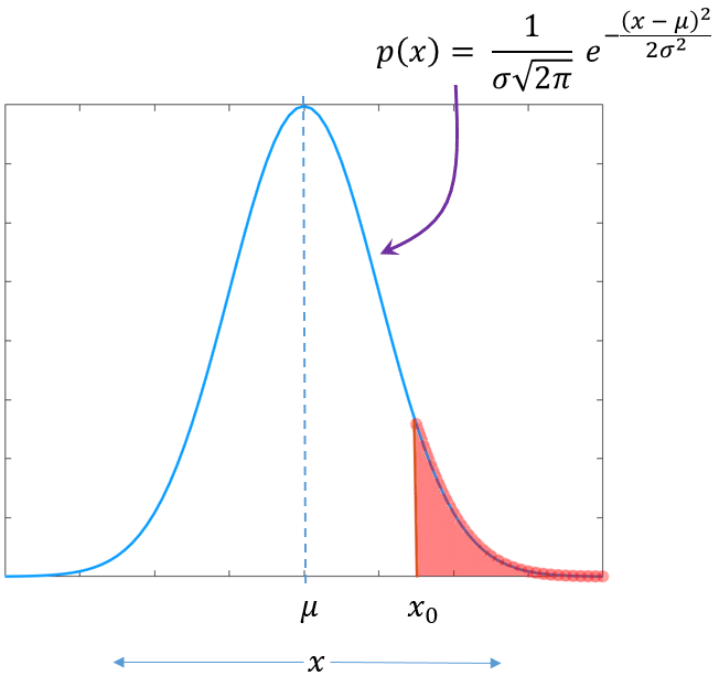
Gaussian PDF with right tail shaded — the Q-function — Figure 1: Standard picture of $latex Q(\cdot) $: area of the right tail beyond the decision threshold.

That probability is

\[\Pr(X \ge x_0) = \int_{x_0}^{\infty} p(x)\,dx \qquad (2)\]

The antiderivative is not elementary. Standardize with $latex y=(x-\mu)/\sigma $:

\[\Pr\!\left(y \ge \frac{x_0-\mu}{\sigma}\right) = \int_{(x_0-\mu)/\sigma}^{\infty} \frac{1}{\sqrt{2\pi}}\,e^{-y^2/2}\,dy \qquad (3)\]

By definition the Q-function is the standard-normal right tail

\[Q(z) = \int_{z}^{\infty} \frac{1}{\sqrt{2\pi}}\,e^{-y^2/2}\,dy \qquad (4)\]

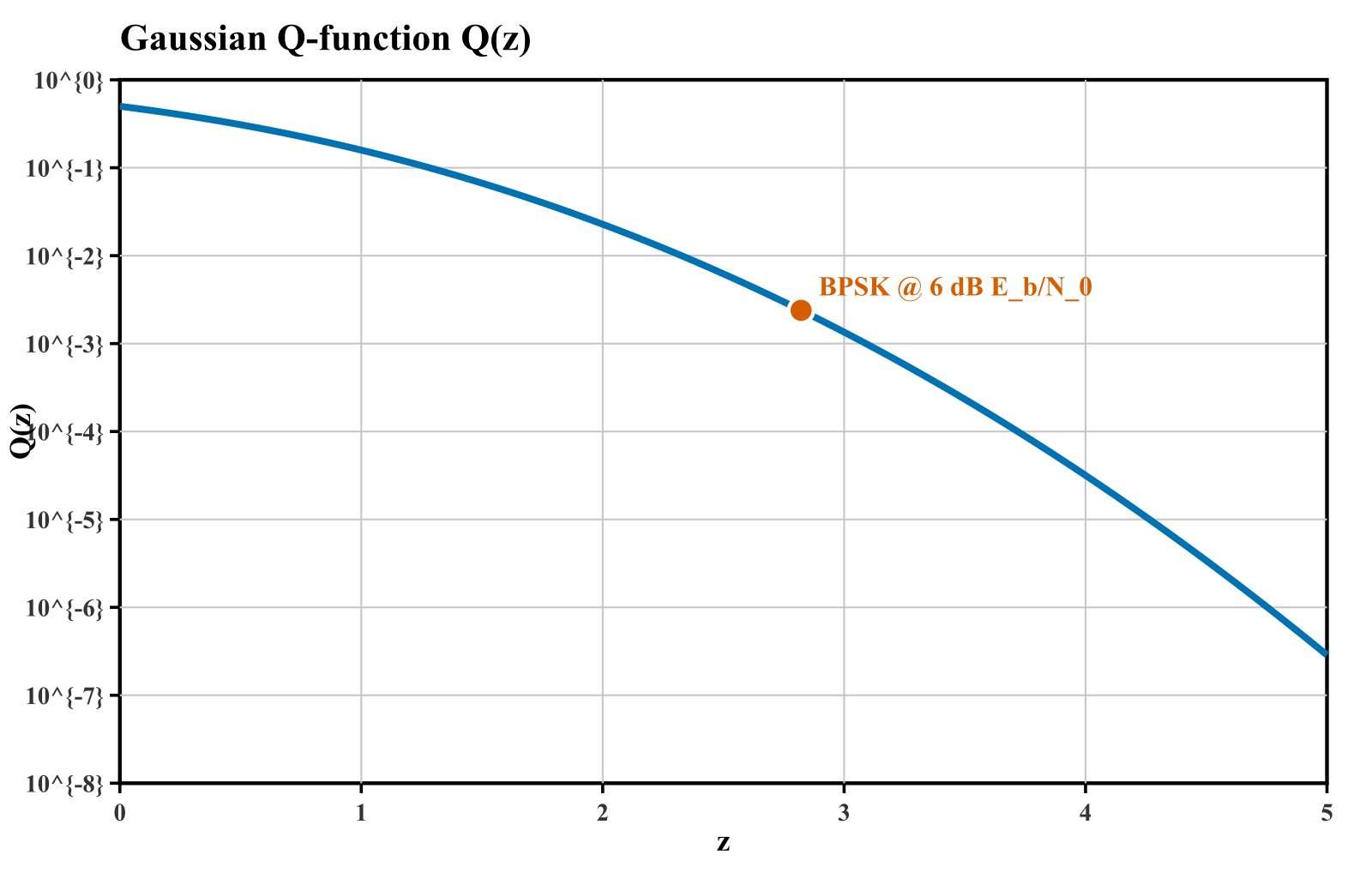
\[\Pr(X \ge x_0) = Q\!\left(\frac{x_0-\mu}{\sigma}\right) \qquad (5)\]

Figure 2 plots $latex Q(z) $ on a log scale — the “waterfall” shape you see in every BER chart.

Gaussian Q-function Q(z) on a log scale with BPSK operating point at 6 dB Eb/N0 — Figure 2: $latex Q(z) $ vs (z). Orange marker: coherent BPSK at $latex E_b/N_0=6\,\mathrm{dB}$, where the argument is $latex z=\sqrt{2E_b/N_0}$.

Error function and complementary error function

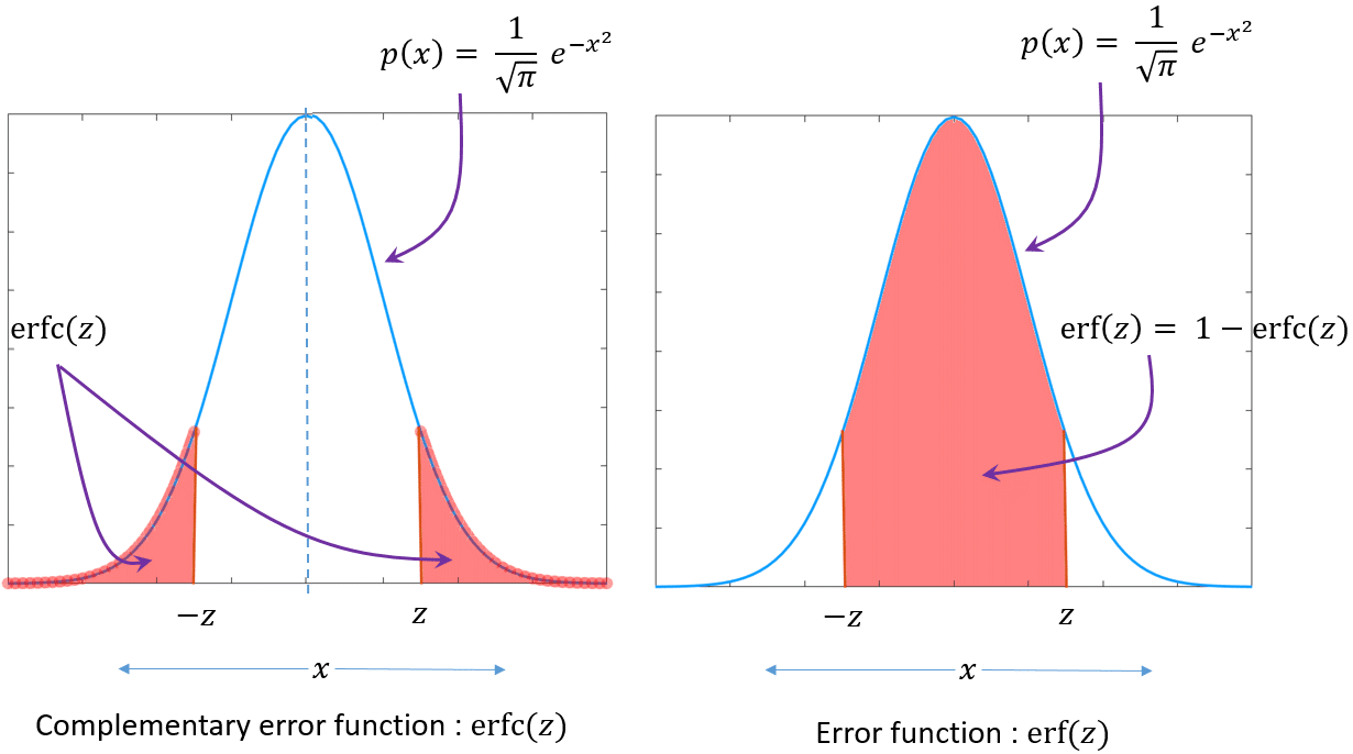
Math libraries and older papers prefer $latex erf $ / $latex erfc $, which use a slightly different Gaussian (variance $latex 1/2 $ instead of $latex 1 $). Geometrically (Figure 2):

$latex erfc(z) $ — for $X\sim\mathcal{N}(0,1/2)$, the two-tail probability $\Pr(|X|>z)$.
$latex erf(z) $ — the complementary central mass $\Pr(|X|<z)=1-erfc(z)$. The integral form runs from $0$ to $z$ because of even symmetry.

Gaussian PDF illustrating erf versus erfc regions — Figure 3: (erf) (central mass) vs $latex erfc $ (complementary tails) under the error-function normalization.

\[erfc(z) = \frac{2}{\sqrt{\pi}}\int_{z}^{\infty} e^{-x^2}\,dx \qquad (6)\] \[erf(z) = 1 – erfc(z) = \frac{2}{\sqrt{\pi}}\int_{0}^{z} e^{-x^2}\,dx \qquad (7)–(8)\]

Conversion: Q ↔ erfc

Matching the integral limits gives the identity every BER derivation uses:

\[Q(z) = \tfrac{1}{2}\,erfc\!\left(\frac{z}{\sqrt{2}}\right) \qquad\Leftrightarrow\qquad erfc(x) = 2\,Q\!\left(x\sqrt{2}\right) \qquad (9)\]

So if a paper writes $latex P_b = \frac{1}{2}\mathrm{erfc}\sqrt{E_b/N_0} $ and another writes $latex P_b = Q\sqrt{2E_b/N_0} $, they are identical for coherent BPSK in AWGN.

Handy identities for BER work

For $latex X \sim \mathcal{N}(\mu,\sigma^2) $:

\[Pr(X \gt x) = Q \left(\frac{x-\mu}{\sigma}\right) \quad (10) \] \[\Pr(X \gt \mu+a) = \Pr(X \lt \mu-a) = Q(a/\sigma) \quad (11)\] \[\Pr(|X-\mu| \gt a) = 2\,Q(a/\sigma) \quad (12)\]

Python: Q, erfc, and a BPSK check

Use SciPy’s ndtr / erfc (or NumPy’s erfc). The snippet below reproduces equation (9) and the coherent-BPSK point marked in Figure 3.

import numpy as np
from math import erfc, sqrt

def Q(z):
    """Standard-normal right-tail probability."""
    return 0.5 * erfc(z / sqrt(2.0))

# Identity (9)
z = np.linspace(0, 4, 9)
assert np.allclose(Q(z), 0.5 * np.erfc(z / np.sqrt(2)))

# Coherent BPSK in AWGN: Pb = Q(sqrt(2 Eb/N0))
ebn0_db = 6.0
ebn0 = 10 ** (ebn0_db / 10)
pb = Q(np.sqrt(2 * ebn0))
print(f"BPSK Pb @ {ebn0_db} dB ≈ {pb:.3e}")
# Cross-check on the live plotter:
# https://www.gaussianwaves.com/tools/ber-ebn0-calculator/?ebn0=6&mod=bpsk

Open the same operating point on the interactive tool: BER vs Eb/N0 calculator (URL state is shareable).

Where this shows up next

Optimum BPSK receiver in AWGN — derives $latex P_b=Q(\sqrt{2E_b/N_0}) $ from first principles.
BPSK BER simulation (Python/Matlab) — Monte Carlo vs the Q-curve.
BPSK on Rayleigh vs AWGN — same Q building block, different average.
Eb/N0, Es/N0, SNR conversions — keep units straight before calling $latex Q(\cdot) $.

FAQ

How are the Q-function, erf, and erfc related? They describe the same Gaussian tail probability with different normalizations. In communications we usually write bit-error rates with $latex Q(x)=\tfrac12\mathrm{erfc}(x/\sqrt{2})$, while many math libraries expose erf/erfc directly. Once you can convert among them, any textbook BER formula becomes interchangeable.

Why do so many BER formulas use Q instead of erfc? The Q-function is the right-tail probability of a standard normal random variable, which matches the geometry of a threshold test in AWGN: the decision statistic is Gaussian, and an error occurs when noise pushes it across the threshold. That probabilistic reading is more direct than the error-function integral used in pure mathematics.

Where do I use this for BPSK? Coherent BPSK in AWGN has $latex P_b=Q(\sqrt{2E_b/N_0})$. The BPSK article and BER calculator use the same expression so you can check simulation points against theory.