Introduction to Probability: The Foundation of Random Signals
In the world of communication engineering, “certainty” is a luxury we don’t have. From the thermal noise in your smartphone’s receiver to the fading of a satellite signal, every process we analyze is governed by uncertainty.
Probability is the mathematical language that allows us to model these random events. It is the reason we can predict that a system will work “99.99% of the time,” even if we can’t predict exactly what the next noise voltage sample will be.
Basic Terminology
- Random Experiment: Any process where the outcome is not known in advance (e.g., measuring the voltage of a noise source).
- Sample Space ($S$): The set of all possible outcomes of an experiment.
- Random Variable ($X$): A mapping that assigns a numerical value to each outcome in the sample space.
Characterizing Randomness: The CDF and PDF
To make engineering decisions, we need functions that describe how “likely” certain values are.
The Cumulative Distribution Function (CDF)
The CDF, denoted by $F_X(x)$, tells us the probability that a random variable $X$ will take a value less than or equal to a specific value $x$.
$$F_X(x) = P(X \leq x)$$
Key Properties:
- The value of a CDF is always between 0 and 1.
- It is a non-decreasing function.
- As $x \to \infty$, $F_X(x) \to 1$.
The Probability Density Function (PDF)
While the CDF tells us about accumulation, the PDF ($f_X(x)$) tells us about the “density” of probability at a specific point. For continuous variables, the PDF is the derivative of the CDF:
$$f_X(x) = \frac{d}{dx} F_X(x)$$
If you want to find the probability that a signal falls between two levels, $a$ and $b$, you calculate the area under the PDF curve:
$$P(a \leq X \leq b) = \int_{a}^{b} f_X(x) \, dx$$
The Gaussian Distribution (The “Normal” Case)
The most important distribution for this site is the Gaussian (Normal) Distribution. In any electronic system, thermal noise is the result of millions of tiny, independent movements of electrons. According to the Central Limit Theorem, the sum of these independent events results in a Gaussian PDF.
The PDF of a Gaussian random variable with mean $\mu$ and variance $\sigma^2$ is:
$$f(x) = \frac{1}{\sigma \sqrt{2\pi}} \exp\left( -\frac{(x – \mu)^2}{2\sigma^2} \right)$$
Why Engineers Love the Gaussian:
In Gaussian noise, the “Mean” represents the DC component, and the “Variance” ($\sigma^2$) represents the average noise power. This direct link between statistics and physics is why the Gaussian model is the industry standard for AWGN (Additive White Gaussian Noise) channels.
Why This Matters for Communication Systems
You might wonder why we need these integrals. Here is how they translate to real-world engineering:
| Statistical Concept | Engineering Metric |
| PDF Area (Tail) | Bit Error Rate (BER) |
| Mean ($\mu$) | Signal DC Level / Offset |
| Variance ($\sigma^2$) | Noise Power |
| PDF Shape | Signal-to-Noise Ratio (SNR) Requirements |
Here is the “Cheat Sheet” reference block for your WordPress post. It is formatted with clean LaTeX and structured for quick reference by engineers and students.
Common Probability Distributions in Communications
In communication theory, choosing the right statistical model is half the battle. Use this table as a quick guide to selecting the distribution that best fits your channel or noise model.
Summary Table of Distributions
| Distribution | Physical Application | Key Parameters |
| Gaussian (Normal) | Thermal Noise (AWGN), sum of many small random effects. | $\mu$ (Mean), $\sigma^2$ (Variance) |
| Uniform | Quantization noise in ADC/DAC, phase of a carrier. | $a$ (Lower bound), $b$ (Upper bound) |
| Rayleigh | Fading in Non-Line-of-Sight (NLOS) wireless channels. | $\sigma$ (Scale parameter) |
| Rician | Fading in Line-of-Sight (LOS) wireless channels. | $\nu$ (LOS component), $\sigma$ (Scatter) |
PDF Formulas
Gaussian Distribution
Used for modeling electronic thermal noise and the majority of background interference.
$$f(x) = \frac{1}{\sigma \sqrt{2\pi}} \exp\left( -\frac{(x – \mu)^2}{2\sigma^2} \right)$$
Uniform Distribution
Typically used to model the error introduced by digitizing a signal (Quantization Noise) or a random phase offset.
$$f(x) = \begin{cases} \frac{1}{b – a} & \text{for } a \leq x \leq b \\ 0 & \text{otherwise} \end{cases}$$
Rayleigh Distribution
The standard model for “Flat Fading” in mobile communications where there is no direct line-of-sight between the transmitter and receiver.
$$f(x) = \frac{x}{\sigma^2} \exp\left( -\frac{x^2}{2\sigma^2} \right), \quad x \geq 0$$
Rician Distribution
A more complex version of Rayleigh used when a strong “specular” or direct Line-of-Sight (LOS) path exists alongside multi-path scattering.
$$f(x) = \frac{x}{\sigma^2} \exp\left( -\frac{x^2 + \nu^2}{2\sigma^2} \right) I_0\left( \frac{x\nu}{\sigma^2} \right), \quad x \geq 0$$
Note: $I_0(\cdot)$ is the modified Bessel function of the first kind, zeroth order.
Here is the Python script to visualize the comparison between the four primary probability distributions.
Python Script: PDF Comparison Plot
This script uses scipy.stats to generate and overlay the four PDFs, providing a visual reference for how probability “spreads” differently across each model.
import numpy as np
import matplotlib.pyplot as plt
from scipy.stats import norm, uniform, rayleigh, rice

# Define the range for the x-axis
x = np.linspace(-2, 10, 1000)

# 1. Gaussian: Mean=4, Std=1.5
pdf_gaussian = norm.pdf(x, loc=4, scale=1.5)

# 2. Uniform: From 1 to 7
pdf_uniform = uniform.pdf(x, loc=1, scale=6)

# 3. Rayleigh: Scale=2.5
pdf_rayleigh = rayleigh.pdf(x, scale=2.5)

# 4. Rician: Non-centrality (nu)=3.5, Scale=1.5
pdf_rician = rice.pdf(x, b=3.5/1.5, scale=1.5)

# Plotting
plt.figure(figsize=(10, 6))
plt.plot(x, pdf_gaussian, 'b-', lw=2, label='Gaussian (Normal)')
plt.plot(x, pdf_uniform, 'g--', lw=2, label='Uniform')
plt.plot(x, pdf_rayleigh, 'r-.', lw=2, label='Rayleigh')
plt.plot(x, pdf_rician, 'm:', lw=2, label='Rician')

plt.title('Comparison of Probability Density Functions (PDFs)')
plt.xlabel('Value (x)')
plt.ylabel('Probability Density')
plt.legend()
plt.grid(True, linestyle=':', alpha=0.7)
plt.ylim(0, 0.45)
plt.show()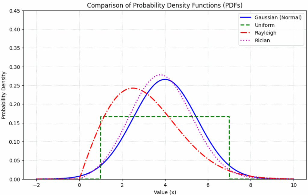
The Engineer’s Dilemma
The Gaussian distribution, often called the “bell-shaped curve,” holds a unique, almost mystical status in communications. Its prominence isn’t just a matter of convenience; it satisfies several optimal criteria that make it the bedrock of signal processing. While Abraham De Moivre first discovered it in 1733, it was later rediscovered by Gauss and Laplace, eventually leading to the Central Limit Theorem (CLT). The CLT explains why Gaussianity is ubiquitous: it is the natural result of many independent random variables acting together—such as the millions of electrons moving in a circuit to create thermal noise.
The Marvels of Symmetry and Invariance
One of the most fascinating properties of the Gaussian shape is its invariance under Fourier transformation. In simpler terms, a Gaussian pulse in the time domain remains a Gaussian pulse in the frequency domain. This makes it an “eigenfunction” of the Fourier transform—a rare trait shared by very few other functions. Furthermore, Gaussian pulses possess the smallest possible time-bandwidth product, meaning they are perfectly concentrated in both time and frequency domains simultaneously. This is why Gaussian filters are the standard choice for intermediate frequency stages in spectrum analyzers.
The “Noisiest” and “Worst-Case” Waveform
In the realm of Information Theory, Gaussian noise is both the “most random” and the most challenging impairment.
- Maximum Entropy: For a fixed variance, the Gaussian distribution maximizes differential entropy, making it the “noisiest” possible waveform.
- Minimum Capacity: Paradoxically, it represents the “worst-case” scenario for communication. Among all channels with additive noise of a fixed power, Gaussian noise yields the smallest channel capacity.
By designing codes that can survive under these “worst-case” Gaussian conditions, engineers ensure a conservative and robust system that will perform reliably in almost any real-world environment.
Summary
Probability isn’t just about rolling dice; it’s about modeling the invisible forces (noise, interference, and fading) that degrade our signals. By mastering the PDF and CDF, you gain the ability to quantify the reliability of any communication link. We love the Gaussian distribution because it makes our linear system math easy (since a Gaussian process remains Gaussian after passing through a linear system), but we respect it because it represents the most difficult noise environment we have to overcome.
Reference :
[1] S.Pasupathy, “Glories of Gaussianity”, IEEE Communications magazine, Aug 1989 – 1, pp 38.
It will be better to go in more details like stochastic process
Ya I can deal with Random process in detail but I think divulging to finer details of Random process itself will need a separate blog.
GREAT EFFORT!!! JAzak Allah kol khayr
GREAT EFFORT!!! JAzak Allah kol khayr
how can we quantify(measure) gaussian white noise in image using matlab,(donot want to use PSNR)
I am not sure about image processing. However, this link might help
http://www.mathworks.com/help/images/ref/imnoise.html
Hello , your website is a great help for topic understanding and implementing in our project .
Sir can you plz give me the simplest PDF and CDF vs Capacity matlab code for mimo system without channel matrix ??
I mean i m using simulink platform and H matrix need not be in the code for the plot..
hoping for your fast reply at [email protected]
sir, please help me……i want to write a MATLAB script which generates N
samples from a Rayleigh distribution, and compares the sample histogram with the
Rayleigh density function. but i want to take starting point as given script
mu = 0; % mean (mu)
sig = 2; % standard deviation (sigma)
N = 1e5; % number of samples
% Sample from Gaussian distribution %
z = mu + sig*randn(1,N);
% Plot sample histogram, scaling vertical axis
%to ensure area under histogram is 1
dx = 0.5;
x = mu-5*sig:dx:mu+5*sig; % mean, and 5 standard
% deviations either side
H = hist(z,x);
area = sum(H*dx);
H = H/area;
bar(x,H)
xlim([-5*sig,5*sig])
% Overlay Gaussian density function
hold on
f = exp(-(x-mu).^2/(2*sig^2))/sqrt(2*pi*sig^2);
plot(x,f,’r’,’LineWidth’,3)
hold off
Please check this post. It has the complete code.
https://www.gaussianwaves.com/2010/02/fading-channels-rayleigh-fading-2/
Thank you….. I’ll follow. but confuse on how to start from this script….will try it.