Eb/N0, Es/N0 and SNR — conversions for BER simulations

In one sentence: Bit-error-rate theory is almost always written against $latex E_b/N_0$, but your simulator adds noise against a symbol energy $latex E_s$ (and a sampling-rate convention). This article derives the exact conversions among $latex E_b/N_0$, $latex E_s/N_0$, and SNR, then shows how to generate complex baseband AWGN so Monte Carlo curves overlay the textbook formula.

If a student’s simulated BER curve sits neatly below theory, or looks “too good” by a few dB, the first place to look is not the demodulator: it is the noise variance. Mixing up $latex E_b$ and $latex E_s$, forgetting the factor of two between real and complex noise, or ignoring oversampling are the classic mistakes. Master those and the rest of a BER lab becomes much calmer.

1. What $latex E_b$, $latex E_s$, and $latex N_0$ actually mean

Start from continuous-time complex baseband. A digital transmitter emits a sequence of symbols $latex \{s[m]\}$ through a pulse $latex p(t)$ of symbol period $latex T$. The average energy carried by one modulation symbol (after the pulse is normalized appropriately) is $latex E_s$. If each symbol conveys $latex k=\log_2 M$ information bits — for example $latex k=1$ for BPSK, $latex k=2$ for QPSK, $latex k=4$ for 16-QAM — then the average energy per information bit is

$latex E_b = E_s / k$.

Additive white Gaussian noise is characterized by a one-sided power spectral density $latex N_0$ (watts per hertz). In the equivalent complex baseband model the noise is circularly symmetric complex Gaussian with two-sided PSD $latex N_0$ total for the complex envelope (that is, $latex N_0/2$ in each of the in-phase and quadrature dimensions). The dimensionless ratios

$latex \displaystyle \gamma_b = \frac{E_b}{N_0}, \qquad \gamma_s = \frac{E_s}{N_0}$

are the fundamental SNRs of digital communications. Almost every closed-form AWGN BER or SER formula in a textbook is written in terms of $latex \gamma_b$ or $latex \gamma_s$.

The conversion that every simulator needs

Because $latex E_s = k E_b$, the two ratios differ only by the bits-per-symbol factor:

$latex \displaystyle \frac{E_s}{N_0} = k\,\frac{E_b}{N_0}$.

In decibels this becomes a simple offset:

$latex \displaystyle \left.\frac{E_s}{N_0}\right|_{\mathrm{dB}} = \left.\frac{E_b}{N_0}\right|_{\mathrm{dB}} + 10\log_{10} k$.

Numerically: QPSK ($latex k=2$) sits $latex 10\log_{10}2 \approx 3.01$ dB above BPSK on an $latex E_s/N_0$ axis for the same $latex E_b/N_0$; 16-QAM ($latex k=4$) sits about $latex 6.02$ dB above BPSK. The figure below plots that family of lines.

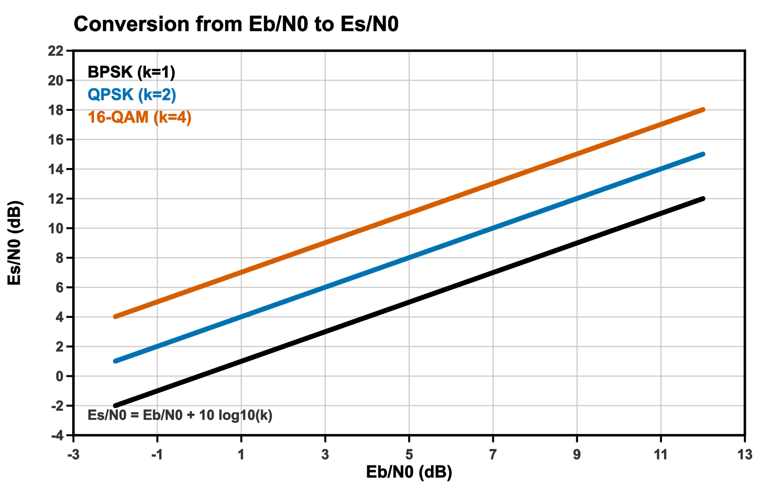
A crucial pedagogical point: for coherent BPSK and Gray-coded QPSK in AWGN, the bit-error rate versus $latex E_b/N_0$ is identical. That does not mean the noise variances in a QPSK and a BPSK simulator are the same when you sweep $latex E_b/N_0$. The QPSK symbol carries two bits, so for a fixed $latex E_b$ the symbol energy is twice as large, and the noise variance you attach to each QPSK symbol must be set from $latex E_s/N_0 = 2\,E_b/N_0$.

2. SNR: one word, several definitions

“SNR” is overloaded. In this article we reserve it for the ratio of average signal power to average noise power in the discrete-time observation the detector actually uses. Under the unit-energy complex-baseband convention of the next section, that SNR equals $latex E_s/N_0$ at one sample per symbol. In an RF receiver chain, “SNR” might instead mean carrier-to-noise ratio in a stated resolution bandwidth, before matched filtering. Always write down which definition you mean.

Related quantities you will meet:

• CNR / C/N — carrier power over noise power in a RF bandwidth $latex B$. Related to $latex E_s/N_0$ once you know the symbol rate and how much of $latex B$ the matched filter uses.
• SNR per bit — another name for $latex E_b/N_0$.
• SNR per sample — after oversampling, before the matched filter; smaller than $latex E_s/N_0$ by roughly the oversampling factor if noise is white.

3. Complex baseband AWGN with unit-energy symbols

Most educational Monte Carlo loops work with discrete symbols $latex s[m] \in \mathbb{C}$ normalized so that

$latex E\big[|s[m]|^2\big] = 1$.

For QPSK that means the four constellation points lie on the unit circle (or on a square scaled by $latex 1/\sqrt{2}$). For M-QAM one scales the rectangular grid so the average power over the constellation is one.

We want the received sample $latex r = s + n$ to satisfy

$latex \displaystyle \frac{E\big[|s|^2\big]}{E\big[|n|^2\big]} = \gamma_s = \frac{E_s}{N_0}$.

With $latex E[|s|^2]=1$ this forces $latex E[|n|^2] = 1/\gamma_s$. Circularly symmetric complex Gaussian noise with that power is written

$latex n \sim \mathcal{CN}(0,\sigma^2), \qquad \sigma^2 = 1/\gamma_s$.

In practice one draws two independent real standard normals $latex n_I, n_Q \sim \mathcal{N}(0,1)$ and sets

$latex \displaystyle n = \sqrt{\frac{\sigma^2}{2}}\,(n_I + j n_Q) = \frac{1}{\sqrt{2\gamma_s}}\,(n_I + j n_Q)$.

The factor $latex 1/\sqrt{2}$ assigns half the noise power to I and half to Q, which is exactly what circular symmetry requires. If you omit it and put variance $latex \sigma^2$ into each of I and Q, you inject twice as much noise and your BER curve will look about 3 dB too pessimistic.

From a plotted $latex E_b/N_0$ to the noise variance

In a BER sweep the horizontal axis is almost always $latex E_b/N_0$ in dB. The algorithm is:

• Convert $latex (E_b/N_0)_{\mathrm{dB}}$ to linear: $latex \gamma_b = 10^{(E_b/N_0)_{\mathrm{dB}}/10}$.
• Form $latex \gamma_s = k\,\gamma_b$.
• Set $latex \sigma^2 = 1/\gamma_s$ for unit-energy symbols.
• Draw $latex n$ as above and compute $latex r = s + n$.

Worked example: QPSK at $latex E_b/N_0 = 6$ dB. Then $latex \gamma_b = 10^{0.6} \approx 3.981$, $latex k=2$, so $latex \gamma_s \approx 7.962$ (about $latex 9.01$ dB). The complex noise variance is $latex \sigma^2 \approx 0.1256$, and each of I and Q is scaled by $latex \sqrt{\sigma^2/2} \approx 0.2506$.

4. Reference implementations (Python and Matlab)

The following Python helper adds complex AWGN when symbols are already unit-energy and the SNR axis is $latex E_b/N_0$ in dB. Read the docstring carefully: if your constellation is not unit-energy, either normalize it or multiply $latex \sigma^2$ by the actual $latex E[|s|^2]$.

import numpy as np

def awgn_complex(signal, ebn0_db, bits_per_symbol):
    """
    Add circularly symmetric complex AWGN.

    Parameters
    ----------
    signal : ndarray (complex)
        Transmitted symbols with E[|s|^2] = 1.
    ebn0_db : float
        Desired Eb/N0 in decibels (the BER plot axis).
    bits_per_symbol : int
        k = log2(M). Use 1 for BPSK, 2 for QPSK, 4 for 16-QAM, etc.

    Returns
    -------
    ndarray
        Noisy observations r = s + n with E[|n|^2] = 1 / (k * Eb/N0_linear).
    """
    ebn0_lin = 10 ** (ebn0_db / 10.0)
    esn0_lin = ebn0_lin * bits_per_symbol
    sigma2 = 1.0 / esn0_lin
    noise = np.sqrt(sigma2 / 2.0) * (
        np.random.randn(*signal.shape) + 1j * np.random.randn(*signal.shape)
    )
    return signal + noise


# Demo: unit-energy Gray QPSK at Eb/N0 = 6 dB
k = 2
bits = np.random.randint(0, 2, size=(20000, k))
idx = bits[:, 0] * 2 + bits[:, 1]
const = np.array([1+1j, -1+1j, -1-1j, 1-1j]) / np.sqrt(2)
s = const[idx]
r = awgn_complex(s, ebn0_db=6.0, bits_per_symbol=k)
emp = np.mean(np.abs(s) ** 2) / np.mean(np.abs(r - s) ** 2)
print("empirical Es/N0 (linear) ~", emp)
print("target Es/N0 (linear)    ~", 2 * 10 ** 0.6)

The same logic in Matlab/Octave:

function r = awgn_complex(s, ebn0_db, k)
% s : complex symbols with mean(abs(s).^2) = 1
ebn0 = 10.^(ebn0_db/10);
esn0 = ebn0 * k;
sigma2 = 1./esn0;
n = sqrt(sigma2/2) .* (randn(size(s)) + 1j*randn(size(s)));
r = s + n;
end

After a long run, the empirical ratio $latex \widehat{E}[|s|^2]/\widehat{E}[|r-s|^2]$ should sit close to the target $latex \gamma_s$. If it does not, the constellation is not unit-energy or the noise scaling is wrong.

5. Real baseband (BPSK on a single rail)

If you simulate real BPSK with $latex s[m] \in \{\pm 1\}$ and real noise only, the model is $latex n \sim \mathcal{N}(0, \sigma^2)$ with $latex \sigma^2 = N_0/(2E_s)$ in the classical matched-filter derivation, which yields $latex P_b = Q(\sqrt{2E_b/N_0})$ for coherent BPSK. Equivalently, with unit-energy real symbols ($latex E[s^2]=1$) set $latex \sigma^2 = 1/(2\gamma_b)$ when the plot axis is $latex E_b/N_0$. Mixing the real formula with a complex noise generator (or vice versa) is another frequent source of 3 dB errors.

6. Oversampling, pulse shaping, and matched filters

Life gets richer once you leave one-sample-per-symbol. Suppose you synthesize a pulse-shaped waveform at $latex L$ samples per symbol and add white discrete-time noise before the receive matched filter. White noise at rate $latex L/T$ has a different per-sample variance than noise at rate $latex 1/T$. A consistent approach:

• Decide the continuous-time PSD $latex N_0$ from the desired $latex E_s/N_0$ and the symbol energy in continuous time.
• Set the discrete-time noise variance per sample to $latex \sigma_{\mathrm{samp}}^2 = N_0 \cdot f_s$ (complex) or $latex N_0 f_s / 2$ per real dimension, with $latex f_s = L/T$.
• After a correctly normalized matched filter and symbol-rate sampling, the decision statistic should again see SNR $latex E_s/N_0$.

If you instead add noise after an ideal matched filter at one sample per symbol, you may use the simple unit-energy formulas of Section 3 directly. Many teaching simulators do exactly that, and it is perfectly valid for AWGN error-rate curves.

7. OFDM and multipath notes

In OFDM the story gains bookkeeping. Unused guard subcarriers, cyclic-prefix overhead, and pilot density all change how transmit energy per information bit relates to the noise variance on a data tone. A clean convention:

• Fix $latex E_b/N_0$ for information bits.
• Account for the fraction of energy spent on CP and pilots when converting to per-active-subcarrier $latex E_s/N_0$.
• Add complex noise per time-domain sample (or per tone after the DFT) with a variance consistent with that $latex E_s/N_0$.

Skipping the CP/pilot overhead term systematically shifts coded BER curves relative to theory. For flat AWGN OFDM without pilots, the conversion of Section 1 still applies per QAM symbol on each data tone.

8. Common pitfalls (and how they move the BER curve)

• Using $latex E_b/N_0$ as if it were $latex E_s/N_0$ for QPSK/QAM. Noise is too weak by a factor $latex k$. The simulated curve sits about $latex 10\log_{10}k$ dB to the left of theory (looks “better” than it should).
• Forgetting the $latex 1/\sqrt{2}$ split between I and Q. Noise power is doubled. The curve sits about 3 dB to the right of theory.
• Non-unit-energy constellations. If $latex E[|s|^2]=P \neq 1$ but you still set $latex \sigma^2=1/\gamma_s$, the true SNR is $latex P\gamma_s$. Either normalize the constellation or use $latex \sigma^2 = P/\gamma_s$.
• Gray vs binary labeling. Does not change noise variance, but it does change BER for a given SER. Compare apples to apples when overlaying theory.
• Too few error events at high SNR. A quiet curve is not a correct curve — increase the bit count until you have enough errors for a stable estimate.

9. How to verify you got it right

For coherent BPSK in AWGN the bit-error probability is

$latex \displaystyle P_b = Q\big(\sqrt{2 E_b/N_0}\big) = \tfrac{1}{2}\mathrm{erfc}\sqrt{E_b/N_0}$.

Generate a Monte Carlo curve with the noise recipe above, overlay this expression (see the Q-function article), and confirm agreement within sampling noise. Then repeat for Gray-coded QPSK: the BER versus $latex E_b/N_0$ should match BPSK, while the noise variance inside the loop must use $latex k=2$. Cross-check individual operating points on the BER vs Eb/N0 calculator.

A second, quick self-check: with unit-energy symbols and no detector, the sample average $latex \widehat{E}[|s|^2]/\widehat{E}[|n|^2]$ must equal the designed $latex E_s/N_0$ to within a few percent on a long vector.

FAQ

Is SNR the same as $latex E_s/N_0$? In the unit-energy, one-sample-per-symbol complex baseband model of Section 3, yes: the decision-statistic SNR is exactly $latex E_s/N_0$. In RF test reports, “SNR” may refer to a different bandwidth or to a measurement before matched filtering — state the definition whenever you leave the discrete symbol model.

Why do textbooks plot BER against $latex E_b/N_0$ rather than $latex E_s/N_0$? Because $latex E_b/N_0$ measures energy cost per information bit, which is the fair currency when comparing constellations that carry different numbers of bits per symbol. Two modulations with the same $latex E_s/N_0$ are not equally efficient if one carries more bits.

Does Gray-coded QPSK really have the same BER as BPSK? Yes, versus $latex E_b/N_0$ in coherent AWGN. Each QPSK symbol is two independent BPSK symbols on orthogonal carriers; Gray labeling ensures nearest-neighbor symbol errors flip a single bit. The noise variance in the simulator still depends on $latex k=2$ when the axis is $latex E_b/N_0$.

How do I include coding rate $latex R$? With a rate-$latex R$ channel code, information-bit energy and channel-bit energy differ: $latex E_b^{\mathrm{info}}/N_0 = (E_s/N_0)/(kR)$ when $latex k$ coded bits ride on each symbol. Sweeping “$latex E_b/N_0$” without specifying whether $latex b$ means information or coded bits is a classic ambiguity in coded BER papers — define it explicitly.

Where should I go next? Implement noise with the AWGN generation article, run a full sweep in the BPSK BER simulation walk-through, and keep the BER calculator open as an oracle for theoretical points.

Similar articles

• Q-function, erf, and erfc
• BPSK modulation and demodulation
• QPSK modulation and demodulation
• Generate AWGN without awgn()
• BPSK BER simulation (Python/Matlab)
• BER vs Eb/N0 calculator