Doppler Spread and Coherence Time Explained with Simulation

Mobile wireless channels change over time. A phone walking or driving changes the paths its signal takes, and that makes the received signal strength and phase jump around. Two quantities describe this behaviour: the Doppler spread, which describes how much the frequency of the signal is smeared, and the coherence time, which describes how long the channel stays roughly the same. This post explains both from first principles, then shows a short simulation you can run and change yourself.

What you need to know first

• Frequency and wavelength. A carrier at frequency $f$ has wavelength $\lambda = c/f$, where $c = 3 \times 10^8$ m/s. At 2 GHz, $\lambda = 0.15$ m.
• Multipath. A radio signal rarely travels in a straight line. It bounces off buildings, trees and cars, so the receiver gets several copies (paths) that arrive at different times and angles.
• Fading. The copies add up in phase or out of phase. As the receiver moves, the sum changes, so the received amplitude goes up and down. This is fading. When no single direct path dominates, the amplitude follows a Rayleigh distribution.
• Units. Speeds must be in metres per second. 60 km/h = 60 / 3.6 = 16.7 m/s.

Why a moving receiver sees a different frequency

Picture a transmitter sending one wave crest every period. A stationary receiver counts crests at the carrier frequency $f$. Now let the receiver drive toward the transmitter at speed $v$. In each second it moves $v$ metres closer, which is $v/\lambda$ extra wavelengths. So it meets more crests per second:

$$f_{\text{seen}} = f + \frac{v}{\lambda}$$

Moving away gives $f – \frac{v}{\lambda}$. This is the same effect as the change in pitch of a car horn as it passes you. It is the Doppler effect, and it applies to radio waves as much as to sound.

For a general direction, the shift depends on the angle $\theta$ between the direction of motion and the arriving path:

$$f_d = \frac{v}{\lambda}\cos\theta$$

• Head-on, $\theta = 0$ and $\cos\theta = 1$, so the shift is largest.
• Sideways, $\theta = 90 \circ$ and $\cos\theta = 0$, so there is no shift.

The largest possible shift is the maximum Doppler frequency:

$f_m = \frac{v}{\lambda}$

Worked example

A phone moves at 60 km/h on a 2 GHz carrier.

1. Wavelength: $\lambda = \frac{3 \times 10^8}{2 \times 10^9} = 0.15$ m
2. Speed: $v = 60 / 3.6 = 16.7$ m/s
3. Maximum Doppler: $f_m = \frac{16.7}{0.15} \approx 111$ Hz

So the fastest path shifts by 111 Hz, and the slowest by −111 Hz.

Doppler spread

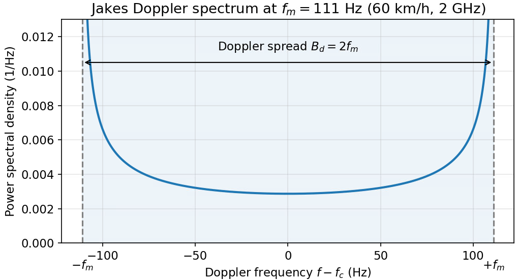
A phone receives many paths from many directions at once. Each path has its own Doppler shift between $-f_m$ and $+f_m$. The range of frequencies that the signal occupies is the Doppler spread.

A common model is the Clarke or Jakes model. Here, scatterers surround the phone and send energy equally from all directions. “Isotropic” simply means “the same in every direction”. The spread then runs from $-f_m$ to $+f_m$, so its total width is:

$$B_d = 2f_m$$

Some textbooks quote $f_m$ alone as the spread. Check which convention a paper uses before you compare numbers.

Coherence time: how long the channel stays the same

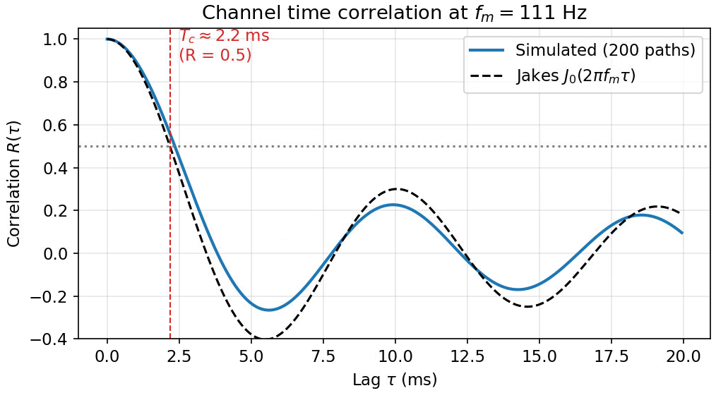
The channel is a random complex number $h(t)$ that changes over time. Correlation asks how similar the channel is at two times separated by a lag $\tau$. The coherence time $T_c$ is the lag at which the correlation falls to a chosen level. This post uses 0.5.

In the Jakes model, the correlation is:

$$R(\tau) = J_0(2\pi f_m \tau)$$

Here $J_0$ is the zero-order Bessel function. You do not need to compute it by hand. It is a standard oscillating function that equals 1 at $\tau = 0$ and falls as $\tau$ grows. Software libraries provide it, for example scipy.special.j0.

The correlation reaches 0.5 when $2\pi f_m \tau \approx 1.52$, which gives:

$$T_c \approx \frac{0.24}{f_m}$$

For the 111 Hz example, $T_c \approx 0.24 / 111 \approx 2.2$ ms.

You will also see the rule of thumb $T_c \approx 0.423/f_m$. It uses a different threshold, so it gives a larger value, about 3.8 ms at 111 Hz. Both are useful. The important part is to state which definition you use.

Typical numbers

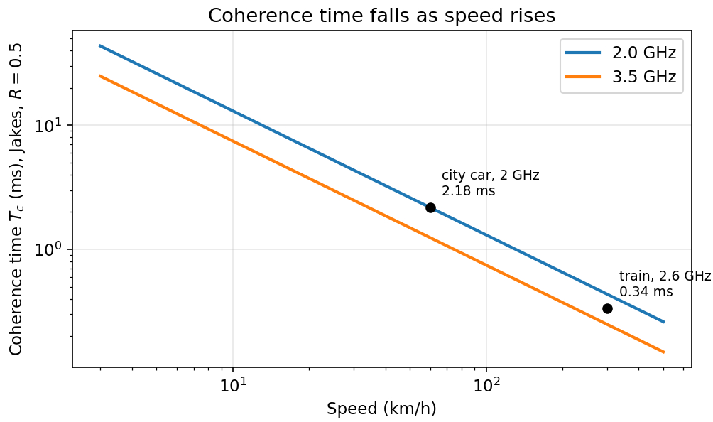
The table uses the Jakes definition ($R = 0.5$) and the rule of thumb side by side.

Simulate it

A Rayleigh fading channel can be built from many sinusoids (the sum-of-sinusoids method). Each sinusoid is one path with:

• a random arrival angle $\theta_n$, which gives its Doppler shift $f_m \cos\theta_n$, and
• a random phase $\phi_n$.

Adding many such terms gives a channel whose correlation follows the Jakes model. The code below builds the channel, measures its correlation, and plots it against the Jakes curve.

import numpy as np
import matplotlib.pyplot as plt
from scipy.special import j0

fs = 20e3                  # sample rate in Hz (one sample every 50 microseconds)
fm = 111.0                 # maximum Doppler frequency in Hz (from the 60 km/h example)
t = np.arange(0, 2, 1/fs)  # time axis: 2 seconds
N = 200                    # number of random paths (more paths give smoother statistics)

rng = np.random.default_rng(1)      # fixed seed, so you get the same result every run
theta = rng.uniform(0, 2*np.pi, N)  # random arrival angle of each path
phi = rng.uniform(0, 2*np.pi, N)    # random phase of each path

# Build the channel by adding one rotating phasor per path
h = np.zeros(len(t), dtype=complex)
for n in range(N):
    doppler_n = fm * np.cos(theta[n])                      # this path's Doppler shift
    h += np.exp(1j*(2*np.pi*doppler_n*t + phi[n]))
h /= np.sqrt(N)                                            # normalise so average power is 1

# Time correlation: average of h(t) * conj(h(t + lag)) over the record
lags = np.arange(400)                                      # lags up to 20 ms
R = np.array([np.mean(h[:len(h)-l] * np.conj(h[l:])) for l in lags]).real
R /= R[0]                                                  # R(0) = 1

Tc = lags[np.argmax(R < 0.5)] / fs                         # first lag where R drops below 0.5
print(f"Coherence time at correlation 0.5: {Tc*1e3:.2f} ms")

# Plot simulation against the Jakes curve
tau = lags / fs
plt.plot(tau*1e3, R, label='simulated')
plt.plot(tau*1e3, j0(2*np.pi*fm*tau), '--', label='Jakes: J0(2 pi fm tau)')
plt.axhline(0.5, color='gray', linestyle=':')
plt.xlabel('lag tau (ms)')
plt.ylabel('correlation')
plt.legend()
plt.grid(True)
plt.show()

import numpy as np
import matplotlib.pyplot as plt
from scipy.special import j0

fs = 20e3                  # sample rate in Hz (one sample every 50 microseconds)
fm = 111.0                 # maximum Doppler frequency in Hz (from the 60 km/h example)
t = np.arange(0, 2, 1/fs)  # time axis: 2 seconds
N = 200                    # number of random paths (more paths give smoother statistics)

rng = np.random.default_rng(1)      # fixed seed, so you get the same result every run
theta = rng.uniform(0, 2*np.pi, N)  # random arrival angle of each path
phi = rng.uniform(0, 2*np.pi, N)    # random phase of each path

# Build the channel by adding one rotating phasor per path
h = np.zeros(len(t), dtype=complex)
for n in range(N):
    doppler_n = fm * np.cos(theta[n])                      # this path's Doppler shift
    h += np.exp(1j*(2*np.pi*doppler_n*t + phi[n]))
h /= np.sqrt(N)                                            # normalise so average power is 1

# Time correlation: average of h(t) * conj(h(t + lag)) over the record
lags = np.arange(400)                                      # lags up to 20 ms
R = np.array([np.mean(h[:len(h)-l] * np.conj(h[l:])) for l in lags]).real
R /= R[0]                                                  # R(0) = 1

Tc = lags[np.argmax(R < 0.5)] / fs                         # first lag where R drops below 0.5
print(f"Coherence time at correlation 0.5: {Tc*1e3:.2f} ms")

# Plot simulation against the Jakes curve
tau = lags / fs
plt.plot(tau*1e3, R, label='simulated')
plt.plot(tau*1e3, j0(2*np.pi*fm*tau), '--', label='Jakes: J0(2 pi fm tau)')
plt.axhline(0.5, color='gray', linestyle=':')
plt.xlabel('lag tau (ms)')
plt.ylabel('correlation')
plt.legend()
plt.grid(True)
plt.show()

In our run it printed about 2.4 ms, close to the Jakes value of 2.2 ms. The random sum means your number will differ a little, and more paths or a longer record make it closer.

What it means for a real link

1. Symbol duration versus coherence time

A transmitter sends symbols of duration $T_s$. If $T_s \ll T_c$, the channel barely changes during one symbol, so one channel estimate per slot is enough.

Example: at 60 km/h, $T_c \approx 2.2$ ms. A 15 kHz OFDM symbol lasts about 67 µs, which is 3% of $T_c$. The channel is effectively static within each symbol.

2. Doppler spread versus subcarrier spacing

OFDM sends data on many subcarriers spaced $\Delta f$ apart (15 kHz in 5G NR, per 3GPP TS 38.211). The subcarriers stay separate only if the channel does not shift them much. A Doppler spread $B_d = 2f_m$ that is large compared with $\Delta f$ smears energy from one subcarrier into its neighbours. This is inter-carrier interference (ICI), and it adds noise-like interference.

Example: a train at 300 km/h on a 2.6 GHz carrier. Here $f_m \approx 722$ Hz and $B_d \approx 1.4$ kHz. That is about 10% of 15 kHz. This is not a hard limit, but at that level 64-QAM starts to suffer, so high-speed systems need more frequent channel estimation or wider subcarrier spacing.

Try it yourself

1. Compute $f_m$ for a train at 300 km/h on a 2.6 GHz carrier. (Answer: about 722 Hz.)
2. In the code, set fm = 722.0 and run it. Predict $T_c$ first using $0.24/f_m$. (Answer: about 0.34 ms. Your simulation should give a similar value.)
3. Why does the correlation fall more slowly at 60 km/h than at 300 km/h? (Answer: $f_m$ is smaller, so the channel changes more slowly.)

Glossary

• Multipath: several copies of a signal arriving by different routes.
• Fading: variation of the received signal caused by the copies adding up in different ways.
• Doppler shift: the change in frequency caused by motion relative to the source of a wave.
• Doppler spread: the range of frequencies the signal occupies because of many Doppler shifts.
• Coherence time: the time over which the channel stays roughly the same.
• OFDM: a modulation that carries data on many closely spaced subcarriers.
• ICI: interference between neighbouring OFDM subcarriers caused by Doppler spread.

Key takeaways

• A moving receiver sees a frequency shift $f_d = (v/\lambda)\cos\theta$, with maximum $f_m = v/\lambda$.
• Doppler spread is $2f_m$ in the Clarke and Jakes model.
• Coherence time is about $0.24/f_m$ at correlation 0.5 (Jakes), or $0.423/f_m$ by the rule of thumb. Always state which one you use.
• Compare the symbol duration with $T_c$, and the Doppler spread with the subcarrier spacing, before you assume a static channel.

For more background, see the Clarke’s Rayleigh fading model post, the Jakes PSD post and Young’s model for Rayleigh fading.