Additionally, 5G NR supports π/2-BPSK in uplink (to be combined with OFDM with CP or DFT-s OFDM with CP)[1][2]. Utilization of π/2-BPSK in the uplink is aimed at providing further reduction of peak-to-average power ratio (PAPR) and boosting RF amplifier power efficiency at lower data-rates.
π/2 BPSK
π/2 BPSK uses two sets of BPSK constellations that are shifted by 90°. The constellation sets are selected depending on the position of the bits in the input sequence. Figure (1) depicts the two constellation sets for π/2 BPSK that are defined as per equation (1)
b[i] = input bits; i = position or index of input bits; d[i] = mapped bits (constellation points)
Figure 1: Two rotated constellation sets for use in π/2 BPSK
Equation (2) is for conventional BPSK – given for comparison. Figure (2) and Figure (3) depicts the ideal constellations and waveforms for BPSK and π/2 BPSK, when a long sequence of random input bits are input to the BPSK and π/2 BPSK modulators respectively. From the waveform, you may note that π/2 BPSK has more phase transitions than BPSK. Therefore π/2 BPSK also helps in better synchronization, especially for cases with long runs of 1s and 0s in the input sequence.
In wireless environments, transmitted signal may be subjected to multiple scatterings before arriving at the receiver. This gives rise to random fluctuations in the received signal and this phenomenon is called fading. The scattered version of the signal is designated as non line of sight (NLOS) component. If the number of NLOS components are sufficiently large, the fading process is approximated as the sum of large number of complex Gaussian process whose probability-density-function follows Rayleigh distribution.
Rayleigh distribution is well suited for the absence of a dominant line of sight (LOS) path between the transmitter and the receiver. If a line of sight path do exist, the envelope distribution is no longer Rayleigh, but Rician (or Ricean). If there exists a dominant LOS component, the fading process can be represented as the sum of complex exponential and a narrowband complex Gaussian process g(t). If the LOS component arrive at the receiver at an angle of arrival(AoA)θ, phase ɸ and with the maximum Doppler frequency fD, the fading process in baseband can be represented as (refer [1])
where, K represents the Rician K factor given as the ratio of power of the LOS component A2 to the power of the scattered components (S2) marked in the equation above.
\[K=\frac{A^2}{S^2}\]
The received signal power Ω is the sum of power in LOS component and the power in scattered components, given as Ω=A2+S2. The above mentioned fading process is called Rician fading process. The best and worst-case Rician fading channels are associated with K=∞ and K=0 respectively. A Ricean fading channel with K=∞ is a Gaussian channel with a strong LOS path. Ricean channel with K=0 represents a Rayleigh channel with no LOS path.
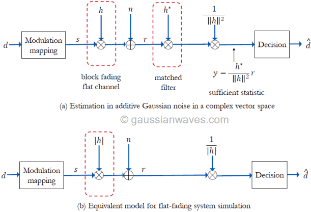
Figure 1: Simulation model for modulation and detection over flat fading channel
Simulation and performance results
In chapter 5 of the book Wireless communication systems in Matlab, the code implementation for complex baseband models for various digital modulators and demodulator are given. The computation and generation of AWGN noise is also given in the book. Using these models, we can create a unified simulation for code for simulating the performance of various modulation techniques over Rician flat-fading channel the simulation model shown in Figure 1(b).
An unified approach is employed to simulate the performance of any of the given modulation technique – MPSK, MQAM or MPAM. The simulation code (given in the book) will automatically choose the selected modulation type, performs Monte Carlo simulation, computes symbol error rates and plots them against the theoretical symbol error rate curves. The simulated performance results obtained for various modulations are shown in the Figure 2.
Figure 2: Performance of various modulations over Ricean flat fading channel
Rate this article: Note: There is a rating embedded within this post, please visit this post to rate it.
This article focused on constructing constellation for rectangular QAM modulation using Karnaugh-map walks. Exploit inherent property of Karnaugh-maps to construct Gray coded QAM constellation points.
Figure 1: Karnaugh-Map walks
Figure 2: Karnaugh-Map walks
M-ary Quadrature Amplitude Modulation (M-QAM)
In MQAM modulations, the information bits are encoded as variations in the amplitude and the phase of the signal. The M-QAM modulator transmits a series of information symbols drawn from the set , with each transmitted symbol holding k bits of information (). To restrict the erroneous receiver decisions to single bit errors, the information symbols are Gray coded. The information symbols are then digitally modulated using a rectangular M-QAM technique, whose signal set is given by
Karnaugh Map Walks and Gray Codes:
In any M-QAM constellation, in order to restrict the erroneous symbol decisions to single bit errors, the adjacent symbols in the transmitter constellation should not differ by more than one bit. This is usually achieved by converting the input symbols to Gray coded symbols and then mapping it to the desired QAM constellation. But this intermediate step can be skipped altogether by using a Look-Up-Table (LUT) approach which properly translates the input symbol to appropriate position in the constellation.
We will exploit the inherent property of Karnaugh Maps to generate the look-up table of dimension (where ) for the gray coded M-QAM constellation which is rectangular and symmetric (M=4, 16, 64, 256, …). The first step in constructing a QAM constellation is to convert a sequential numbers representing the message symbols to gray coded format. The function to convert decimal numbers to Gray codes is given next.
function [grayCoded]=dec2gray(decInput)
%convert decimal to Gray code representation
%example: x= [0 1 2 3 4 5 6 7] %decimal
%y=dec2gray(x); %returns y = [ 0 1 3 2 6 7 5 4] %Gray coded
[rows,cols]=size(decInput);
grayCoded=zeros(rows,cols);
for i=1:rows
   for j=1:cols
    grayCoded(i,j)=bitxor(bitshift(decInput(i,j),-1),decInput(i,j));
   end
end
If you are familiar with Karnaugh Maps (K-Maps) [1], it is easier for you to identify that the K-Maps are constructed based on Gray Codes. By the nature of the construction of K-Maps, the address of the adjacent cells differ by only one bit. If we supper impose the given M-QAM constellation on the K-Map and walk through the address of each cell in certain pattern, it gives the Gray-coded M-QAM constellation.
As mentioned, a walk through the K-Map will produce a sequence of gray codes. Moreover, if the walk can be looped back to the origin or starting point, it will generate a sequence of cyclic Gray codes. Different walking patterns are possible on K-Maps that generate different sequences of Gray codes. Some of the walks on a \(4 \times 4\) K-Map are shown in Figures 1 and 2. This can be readily extended to any K-Map configuration of higher order.
In walk types 1,3 and 4, the address of the starting point and end point differ by only one bit and the corresponding cells are adjacent to each other. In effect, the walk can be looped to give cyclic Gray codes. But in type 2 walk, the starting cell (0000 ) and the ending cell (1101) are not adjacent to each other and thus the Gray code generated using this pattern of walk is not cyclic. By far, type 1 walk is the simplest. All we have to do is alternate the direction of the walk for every row and read the gray coded address.
There exist other constellation shapes (like circular, triangular constellations) that are more efficient (in terms of energy required to achieve same the error probability) than the standard rectangular constellation. Rectangular (symmetric or square) constellations are the preferred choice of implementation due to its simplicity in implementing modulation and demodulation.
Any rectangular QAM constellation is equivalent to superimposing two Amplitude Shift Keying (ASK)signals (also called Pulse Amplitude Modulation – PAM) on quadrature carriers. For example, 16-QAM constellation points can be generated from two 4-PAM signals, similarly the 64-QAM constellation points can be generated from two 8-PAM signals. The generic equation to generate PAM signals of dimension D is
For generating 16-QAM, the dimension D of PAM is set to . Thus for constructing a M-QAM constellation, the PAM dimension is set as . Matlab code for dynamically generating M-QAM constellation points based on Karnaugh map Gray code walk is given below. The resulting ideal constellations for Gray coded 16-QAM and 64-QAM are shown in following figure.
A generic complex baseband simulation technique, to simulate all M-ary QAM modulation techniques is given here. The given simulation code is very generic, and it plots both simulated and theoretical symbol error rates for all M-QAM modulation techniques.
Rectangular QAM from PAM constellation
There exist other constellation shapes (like circular, triangular constellations) that are more efficient (in terms of energy required to achieve same the error probability) than the standard rectangular constellation. Rectangular (symmetric or square) constellations are the preferred choice of implementation due to its simplicity in implementing modulation and demodulation.
Any rectangular QAM constellation is equivalent to superimposing two Amplitude Shift Keying (ASK)signals (also called Pulse Amplitude Modulation – PAM) on quadrature carriers. For example, 16-QAM constellation points can be generated from two 4-PAM signals, similarly the 64-QAM constellation points can be generated from two 8-PAM signals.
Figure 1: Signal space constellations for 16-QAM and 64-QAM
The generic equation to generate PAM signals of dimension D is
For generating 16-QAM, the dimension D of PAM is set to . Thus for constructing a M-QAM constellation, the PAM dimension is set as . Matlab code for dynamically generating M-QAM constellation points based on Karnaugh map Gray code walk is given below. The resulting ideal constellations for Gray coded 16-QAM and 64-QAM are shown in Figure 1.
function [s,ref]=mqam_modulator(M,d)
%Function to MQAM modulate the vector of data symbols - d
%[s,ref]=mqam_modulator(M,d) modulates the symbols defined by the vector d
% using MQAM modulation, where M specifies order of M-QAM modulation and
% vector d contains symbols whose values range 1:M. The output s is modulated
% output and ref represents reference constellation that can be used in demod
if(((M˜=1) && ˜mod(floor(log2(M)),2))==0), %M not a even power of 2
  error('Only Square MQAM supported. M must be even power of 2');
end
  ref=constructQAM(M); %construct reference constellation
  s=ref(d); %map information symbols to modulated symbols
end
class QAMModem(Modem):
    # Derived class: QAMModem

    def __init__(self,M):

        if (M==1) or (np.mod(np.log2(M),2)!=0): # M not a even power of 2
            raise ValueError('Only square MQAM supported. M must be even power of 2')

        n = np.arange(0,M) # Sequential address from 0 to M-1 (1xM dimension)
        a = np.asarray([xˆ(x>>1) for x in n]) #convert linear addresses to Gray code
        D = np.sqrt(M).astype(int) #Dimension of K-Map - N x N matrix
        a = np.reshape(a,(D,D)) # NxN gray coded matrix
        oddRows=np.arange(start = 1, stop = D ,step=2) # identify alternate rows

        nGray=np.reshape(a,(M)) # reshape to 1xM - Gray code walk on KMap
        #Construction of ideal M-QAM constellation from sqrt(M)-PAM
        (x,y)=np.divmod(nGray,D) #element-wise quotient and remainder
        Ax=2*x+1-D # PAM Amplitudes 2d+1-D - real axis
        Ay=2*y+1-D # PAM Amplitudes 2d+1-D - imag axis
        constellation = Ax+1j*Ay
        Modem.__init__(self, M, constellation, name='QAM') #set the modem attributes
Generally the two main categories of detection techniques, commonly applied for detecting the digitally modulated data are coherent detection and non-coherent detection.
In the vector simulation model for the coherent detection, the transmitter and receiver agree on the same reference constellation for modulating and demodulating the information. The modulators generate the reference constellation for the selected modulation type. The same reference constellation should be used if coherent detection is selected as the method of demodulating the received data vector.
On the other hand, in the non-coherent detection, the receiver is oblivious to the reference constellation used at the transmitter. The receiver uses methods like envelope detection to demodulate the data.
The IQ detection technique is an example of coherent detection. In the IQ detection technique, the first step is to compute the pair-wise Euclidean distance between the given two vectors – reference array and the received symbols corrupted with noise. Each symbol in the received symbol vector (represented on a p-dimensional plane) should be compared with every symbol in the reference array. Next, the symbols, from the reference array, that provide the minimum Euclidean distance are returned.
Let x=(x1,x2,…,xp) and y=(y1,y2,…,yp) be two points in p-dimensional space. The Euclidean distance between them is given by
The pair-wise Euclidean distance between two sets of vectors, say x and y, on a p-dimensional space, can be computed using the vectorized code. The vectorized code returns the ideal signaling points from matrix y that provides the minimum Euclidean distance. Since the vectorized implementation is devoid of nested for-loops, the program executes significantly faster for larger input matrices. The given code is very generic in the sense that it can be easily reused to implement optimum coherent receivers for any N-dimensional digital modulation technique (Please refer the books Digital Modulations using Matlab and Digital Modulations using Python for complete simulation code) .
function [dCap]= mqam_detector(M,r)
%Function to detect MQAM modulated symbols
%[dCap]= mqam_detector(M,r) detects the received MQAM signal points
%points - 'r'. M is the modulation level of MQAM
   if(((M˜=1) && ˜mod(floor(log2(M)),2))==0), %M not a even power of 2
      error('Only Square MQAM supported. M must be even power of 2');
   end
   ref=constructQAM(M); %reference constellation for MQAM
   [˜,dCap]= iqOptDetector(r,ref); %IQ detection
end
The simulation results for error rate performance of M-QAM modulations over AWGN channel and Rician flat-fading channel is given in the following figures.
Figure 2: Error rate performance of M-QAM modulations in AWGN channel
This website uses cookies to improve your experience while you navigate through the website. Out of these, the cookies that are categorized as necessary are stored on your browser as they are essential for the working of basic functionalities of the website. We also use third-party cookies that help us analyze and understand how you use this website. These cookies will be stored in your browser only with your consent. You also have the option to opt-out of these cookies. But opting out of some of these cookies may affect your browsing experience.
Necessary cookies are absolutely essential for the website to function properly. These cookies ensure basic functionalities and security features of the website, anonymously.
Cookie
Duration
Description
cookielawinfo-checbox-analytics
11 months
This cookie is set by GDPR Cookie Consent plugin. The cookie is used to store the user consent for the cookies in the category "Analytics".
cookielawinfo-checbox-analytics
11 months
This cookie is set by GDPR Cookie Consent plugin. The cookie is used to store the user consent for the cookies in the category "Analytics".
cookielawinfo-checbox-functional
11 months
The cookie is set by GDPR cookie consent to record the user consent for the cookies in the category "Functional".
cookielawinfo-checbox-functional
11 months
The cookie is set by GDPR cookie consent to record the user consent for the cookies in the category "Functional".
cookielawinfo-checbox-others
11 months
This cookie is set by GDPR Cookie Consent plugin. The cookie is used to store the user consent for the cookies in the category "Other.
cookielawinfo-checbox-others
11 months
This cookie is set by GDPR Cookie Consent plugin. The cookie is used to store the user consent for the cookies in the category "Other.
cookielawinfo-checkbox-necessary
11 months
This cookie is set by GDPR Cookie Consent plugin. The cookies is used to store the user consent for the cookies in the category "Necessary".
cookielawinfo-checkbox-performance
11 months
This cookie is set by GDPR Cookie Consent plugin. The cookie is used to store the user consent for the cookies in the category "Performance".
viewed_cookie_policy
11 months
The cookie is set by the GDPR Cookie Consent plugin and is used to store whether or not user has consented to the use of cookies. It does not store any personal data.
Functional cookies help to perform certain functionalities like sharing the content of the website on social media platforms, collect feedbacks, and other third-party features.
Performance cookies are used to understand and analyze the key performance indexes of the website which helps in delivering a better user experience for the visitors.
Analytical cookies are used to understand how visitors interact with the website. These cookies help provide information on metrics the number of visitors, bounce rate, traffic source, etc.