Key focus: Rectangular pulse shaping with abrupt transitions eliminates intersymbol interference, but it has infinitely extending frequency response. Simulation discussed.
Rectangular pulse
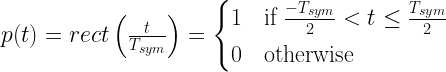
A rectangular pulse with abrupt transitions is a natural choice for eliminating ISI. If an information sequence is shaped as rectangular pulses, at the symbol sampling instants, the interference due to other symbols are always zero. Easier to implement in hardware or software, a rectangular pulse of duration can be generated by the following function
The complete set of Matlab codes to generate a rectangular pulse and to plot the time-domain view and the frequency response is available in the book Wireless Communication Systems in Matlab.
Program 1: rectFunction.m: Function for generating a rectangular pulse
function [p,t,filtDelay]=rectFunction(L,Nsym)
%Function for generating rectangular pulse for the given inputs
%L - oversampling factor (number of samples per symbol)
%Nsym - filter span in symbol durations
%Returns the output pulse p(t) that spans the discrete-time base
%-Nsym:1/L:Nsym. Also returns the filter delay.

Tsym=1;
t=-(Nsym/2):1/L:(Nsym/2); %unit symbol duration time-base
p=(t > -Tsym/2) .* (t <= Tsym/2);%rectangular pulse

%FIR filter delay = (N-1)/2, N=length of the filter
filtDelay = (length(p)-1)/2; %FIR filter delay end
Figure 1: Rectangular pulse and its manifestation in frequency domain
As shown in Figure 1, the rectangular pulse in the time-domain manifests as a sinc function that extends infinitely on either side of the frequency spectrum (though only a portion of the frequency response is plotted in the figure) and thus its spectrum is not band-limited. When the infinitely extending frequency response is stuffed inside a band-limited channel, the truncation of the spectrum leads to energy spills in the time-domain. If we were to use sharp rectangular pulses, it needs a huge bandwidth that could violate practical design specs.
Rate this article: Note: There is a rating embedded within this post, please visit this post to rate it.
Key focus: Baseband communication system and its equivalent DSP implementation (discrete time model) with a pulse shaping & matched filter is briefly introduced.
If a train of pulses representing an information sequence need to be sent across a band-limited dispersive channel, the bandwidth of the channel should be large enough to accommodate the entire spectrum of the signal that is being sent. If we try to stuff the signal spectrum without proper pulse shaping into a band-limited channel, the spectrum of the received signal at the receiver will be truncated by the band-limiting nature of the channel. In time-domain, the energy of one pulse may spill to the time slot allocated for one or more adjacent pulses, leading to Inter-Symbol Interference (ISI) and therefore a source of error in the receiver.
ISI can be minimized by optimal signal design and the detection of a signal with known pulse shape that is buried in noise is a well-studied problem in communication. At the receiver, optimal signal detection is performed by a matched filterwhose impulse response is matched to the impulse response of the pulse shaping filter employed at the transmitter.
A typical baseband communication system and its equivalent DSP implementation (discrete time model) with a matched filter is shown in Figure 1. The interpolating filter at the transmitter is implemented in DSP as a chain of upsampler and a pulse shaping function. The upsampler inserts L-1 zeros between the successive incoming data samples and the pulse shaping filter fills in the zeros generated by the upsampler by using a pulse shaping function. On the other hand, the receiver contains a downsampler that keeps every Lth sample starting from a specified offset. The factor L denotes the oversampling factor or upsampling ratio which is given as the ratio of symbol period (Tsym) and the sampling period (Ts) or equivalently, the ratio of sampling rate Fs and the symbol rate Fsym as
Figure 1: A typical baseband communication system (top) and its equivalent DSP implementation (bottom)
The interpolating filter at the transmitter is implemented in DSP as a chain of upsampler and a pulse shaping function. The upsampler inserts zeros between the successive incoming data samples and the pulse shaping filter fills in the zeros generated by the upsampler by using a pulse shaping function. On the other hand, the receiver contains a downsampler that keeps every sample starting from a specified offset. The factor denotes the oversampling factor or upsampling ratio which is given as the ratio of symbol period () and the sampling period () or equivalently, the ratio of sampling rate and the symbol rate as
The implementation of impulse response of the most widely discussed pulsing shaping functions (filters) will follow in the next series of articles, followed by an example on a complete matched filter system with square-root raised-cosine pulse shaping.
Rate this article: Note: There is a rating embedded within this post, please visit this post to rate it.
The goal of timing recovery is to estimate and correct the sampling instants and phase at the receiver, such that it allows the receiver to decode the transmitted symbols reliably.
What is Symbol timing Recovery :
When transmitting data across a communication system, three things are important: frequency of transmission, phase information and the symbol rate.
In coherent detection/demodulation, both the transmitter and receiver posses the knowledge of exact symbol sampling timing and symbol phase (and/or symbol frequency). While everything is set at the transmitter, the receiver is at the mercy of recovery algorithms to regenerate these information from the incoming signal itself. If the transmission is a passband transmission, the carrier recovery algorithm also recovers the carrier frequency. For phase sensitive systems like BPSK, QPSK etc.., the carrier recovery algorithm recovers the symbol phase so that it is synchronous with the transmitted symbol.
The first part in such a receiver architecture of a MPSK transmitting system is multiplying the incoming signal with sine and cosine components of the carrier wave.
The sine and cosine components are generated using a carrier recovery block (Phase Lock Loop (PLL) or setting a local oscillator to track the variations).
Once the in-phase and quadrature signals are separated out properly, the next task is to match each symbol with the transmitted pulse shape such that the overall SNR of the system improves.
Implementing this in digital domain, the architecture described so far would look like this (Note: the subscript of the incoming signal has changed from analog domain to digital domain – i.e. to )
In the digital architecture above, the matched filter is implemented as a simple finite impulse response (FIR) filter whose impulse response is matched to that of the transmitter pulse shape. It helps the receiver in timing recovery and also it improves the overall SNR of the system by suppressing some amount of noise. The incoming signal up to the point before the matched filter, may have fluctuations in the amplitude. The matched filter also behaves like an averaging filter that smooths out the variations in the signal.
Note that in this digital version, the incoming signal is already a sampled signal. It has already passed through an analog to digital converter that sampled the signal at some sampling rate. From the symbol perspective, the symbols have to be sampled at optimum sampling instant to extract its content properly.
This requires a re-sampler, which resamples the averaged signal at the optimum sampling instant. If the original sampling instant is before or after the optimum sampling point, the timing recovery signal will help to re-sample (re-adjust sampling times) accordingly.
An alternate data pattern (symbols) – [+1,-1,+1,+1,\cdots,] is transmitted across the channel. Assume that each symbol occupies Tsym=8 sample time.
clear all; clc;
n=10; %Number of data symbols
Tsym=8; %Symbol time interms of sample time or oversampling rate equivalently
%data=2*(rand(n,1)<0.5)-1;
data=[1 -1 1 -1 1 -1 1 -1 1 -1]'; %BPSK data
bpsk=reshape(repmat(data,1,Tsym)',n*Tsym,1); %BPSK signal

figure('Color',[1 1 1]);
subplot(3,1,1);
plot(bpsk);
title('Ideal BPSK symbols');
xlabel('Sample index [n]');
ylabel('Amplitude')
set(gca,'XTick',0:8:80);
axis([1 80 -2 2]); grid on;
Lets add white gaussian noise (awgn). A random noise of standard deviation 0.25 is generated and added with the generated BPSK symbols.
noise=0.25*randn(size(bpsk)); %Adding some amount of noise
received=bpsk+noise; %Received signal with noise

subplot(3,1,2);
plot(received);
title('Transmitted BPSK symbols (with noise)');
xlabel('Sample index [n]');
ylabel('Amplitude')
set(gca,'XTick',0:8:80);
axis([1 80 -2 2]); grid on;
From the first plot, we see that the transmitted pulse is a rectangular pulse that spans Tsym samples. In the illustration, Tsym=8. The best averaging filter (matched filter) for this case is a rectangular filter (though they are not preferred in practice, I am just using it for simplifying the illustration) that spans 8 samples. Such a rectangular pulse can be mathematically represented in terms of unit step function as
The resulting rectangular pulse will have a value of 0.5 at the edges of the sampling instants (index 0 and 7) and a value of ‘1’ at the remaining indices in between the edges. Such a rectangular function is indicated below.
The incoming signal is convolved with the averaging filter and the resultant output is given below
We can note that the averaged output peaks at the locations where the symbol transition occurs. Thus, when the signal is sampled at those ideal locations, the BPSK symbols [+1,-1,+1, …] can be recovered perfectly.
But the problem here is: “How does the receiver know the ideal sampling instants?”. The solution is “someone has to supply those ideal sampling instants”. A symbol time recovery circuit is used for this purpose.
Coming back to the receiver architecture, lets add a symbol time recovery circuit that supplies the recovered timing instants. The signal will be re-sampled at those instants supplied by the recovery circuit.
The Algorithm behind Symbol Timing Recovery:
Different algorithms exist for symbol timing recovery and synchronization. An “Early/Late Symbol Recovery algorithm” is illustrated here.
The algorithm starts by selecting an arbitrary sample at some time (denoted by T). It captures the two adjacent samples (on either side of the sampling instant T) that are separated by δ seconds. The sample at the index T-δ is called Early Sample and the sample at the index T+δ is called Late Sample. The timing error is generated by comparing the amplitudes of the early and late samples. The next symbol sampling time instant is either advanced or delayed based on the sign of difference between the early and late sample.
1) If the Early Sample = Late Sample : The peak occurs at the on-time sampling instant T. No adjustment in the timing is needed. 2) If |Early Sample| > |Late Sample| : Late timing, the sampling time is offset so that the next symbol is sampled T-δ/2 seconds after the current sampling time. 3) If |Early Sample| < |Late Sample| : Early timing, the sampling time is offset so that the next symbol is sampled T+δ/2 seconds after the current sampling time.
These three situations are shown next.
There exist many variations to the above mentioned algorithm. The Early/Late synchronization technique given here is the simplest one taken for illustration.
Let’s complete the architecture with a signal quantization and constellation de-mapping block which gives out the estimated demodulated symbols.
Rate this article: Note: There is a rating embedded within this post, please visit this post to rate it.
Note: There is a rating embedded within this post, please visit this post to rate it.
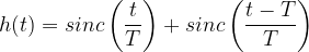
In GMSK modulation (used in GSM and DECT standard), a GMSK signal is generated by shaping the information bits in NRZ format through a Gaussian Filter. The filtered pulses are then frequency modulated to yield the GMSK signal. GMSK modulation is quite insensitive to non-linearities of power amplifier and is robust to fading effects. But it has a moderate spectral efficiency.
An expression for the Gaussian Filter with 3dB Bandwidth is derived here.
The requirements for a gaussian filter used for GMSK modulation in GSM/DECT standard are as follows,
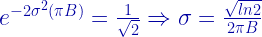
Now the challenge is to design a Gaussian Filter fG(t) that satifies the 3dB bandwidth requirement i.e. in the frequency domain at some frequency f=B, the filter should posses -3dB gain ( in otherwords => half power point located at f=B)
The expression for the required Gaussian Filter can be obtained by choosing the variance of the above mentioned distribution so that the Fourier Transform of the above mentioned expression has a -3dB power gain at f=B.
The fourier transform of the above mentioned expression is
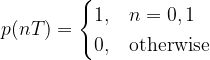
The condition for zero ISI (Inter Symbol Interference) is
which states that when sampling a particular symbol (at time instant nT=0), the effect of all other symbols on the current sampled symbol is zero.
As discussed in the previous article, one of the practical ways to mitigate ISI is to use partial response signaling technique ( otherwise called as “correlative coding”). In partial response signaling, the requirement of zero ISI condition is relaxed as a controlled amount of ISI is introduced in the transmitted signal and is counteracted in the receiver side.
By relaxing the zero ISI condition, the above equation can be modified as,
which states that the ISI is limited to two adjacent samples. Here we introduce a controlled or “deterministic” amount of ISI and hence its effect can be removed upon signal detection at the receiver.
Duobinary Signaling:
The following figure shows the duobinary signaling scheme.
Figure 1: DuoBinary signaling scheme
Encoding Process:
1) an = binary input bit; an ∈ {0,1}. 2) bn = NRZ polar output of Level converter in the precoder and is given by,
3) yn can be represented as
Note that the samples bn are uncorrelated ( i.e either +d for “1” or -d for “0” input). On the other-hand, the samples yn are correlated ( i.e. there are three possible values +2d,0,-2d depending on an and an-1). Meaning that the duobinary encoding correlates present sample an and the previous input sample an-1.
4) From the diagram,impulse response of the duobinary encoder is computed as
Decoding Process:
5) The receiver consists of a duobinary decoder and a postcoder (inverse of precoder).The duobinary decoder implements the following equation (which can be deduced from the equation given under step 3 (see above))
This equation indicates that the decoding process is prone to error propagation as the estimate of present sample relies on the estimate of previous sample. This error propagation is avoided by using a precoder before duobinary encoder at the transmitter and a postcoder after the duobinary decoder. The precoder ties the present sample and previous sample ( correlates these two samples) and the postcoder does the reverse process.
6) The entire process of duobinary decoding and the postcoding can be combined together as one algorithm. The following decision rule is used for detecting the original duobinary signal samples {an} from {yn}
This website uses cookies to improve your experience while you navigate through the website. Out of these, the cookies that are categorized as necessary are stored on your browser as they are essential for the working of basic functionalities of the website. We also use third-party cookies that help us analyze and understand how you use this website. These cookies will be stored in your browser only with your consent. You also have the option to opt-out of these cookies. But opting out of some of these cookies may affect your browsing experience.
Necessary cookies are absolutely essential for the website to function properly. These cookies ensure basic functionalities and security features of the website, anonymously.
Cookie
Duration
Description
cookielawinfo-checbox-analytics
11 months
This cookie is set by GDPR Cookie Consent plugin. The cookie is used to store the user consent for the cookies in the category "Analytics".
cookielawinfo-checbox-analytics
11 months
This cookie is set by GDPR Cookie Consent plugin. The cookie is used to store the user consent for the cookies in the category "Analytics".
cookielawinfo-checbox-functional
11 months
The cookie is set by GDPR cookie consent to record the user consent for the cookies in the category "Functional".
cookielawinfo-checbox-functional
11 months
The cookie is set by GDPR cookie consent to record the user consent for the cookies in the category "Functional".
cookielawinfo-checbox-others
11 months
This cookie is set by GDPR Cookie Consent plugin. The cookie is used to store the user consent for the cookies in the category "Other.
cookielawinfo-checbox-others
11 months
This cookie is set by GDPR Cookie Consent plugin. The cookie is used to store the user consent for the cookies in the category "Other.
cookielawinfo-checkbox-necessary
11 months
This cookie is set by GDPR Cookie Consent plugin. The cookies is used to store the user consent for the cookies in the category "Necessary".
cookielawinfo-checkbox-performance
11 months
This cookie is set by GDPR Cookie Consent plugin. The cookie is used to store the user consent for the cookies in the category "Performance".
viewed_cookie_policy
11 months
The cookie is set by the GDPR Cookie Consent plugin and is used to store whether or not user has consented to the use of cookies. It does not store any personal data.
Functional cookies help to perform certain functionalities like sharing the content of the website on social media platforms, collect feedbacks, and other third-party features.
Performance cookies are used to understand and analyze the key performance indexes of the website which helps in delivering a better user experience for the visitors.
Analytical cookies are used to understand how visitors interact with the website. These cookies help provide information on metrics the number of visitors, bounce rate, traffic source, etc.


![y[n]](https://s0.wp.com/latex.php?latex=y%5Bn%5D&bg=ffffff&fg=000&s=0&c=20201002)


![u[n]-u[n-8]](https://s0.wp.com/latex.php?latex=u%5Bn%5D-u%5Bn-8%5D+&bg=ffffff&fg=000&s=2&c=20201002)


![F[f(t)]=e^{-2 \sigma^{2} ( \pi f) }](https://s0.wp.com/latex.php?latex=F%5Bf%28t%29%5D%3De%5E%7B-2+%5Csigma%5E%7B2%7D+%28+%5Cpi+f%29+%7D&bg=ffffff&fg=0000A0&s=2&c=20201002)