The phase transition properties of the different variants of QPSK schemes and MSK, are easily investigated using constellation diagram. Let’s demonstrate how to plot the signal space constellations, for the various modulations used in the transmitter.
Typically, in practical applications, the baseband modulated waveforms are passed through a pulse shaping filter for combating the phenomenon of intersymbol interference (ISI). The goal is to plot the constellation plots of various pulse-shaped baseband waveforms of the QPSK, O-QPSK and π/4-DQPSK schemes. A variety of pulse shaping filters are available and raised cosine filter is specifically chosen for this demo. The raised cosine (RC) pulse comes with an adjustable transition band roll-off parameter α, using which the decay of the transition band can be controlled.
This article is part of the following books |
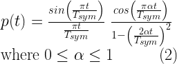
The RC pulse shaping function is expressed in frequency domain as


Equivalently, in time domain, the impulse response corresponds to


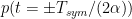
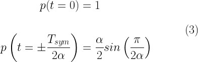
A simple evaluation of the equation (2) produces singularities (undefined points) at p(t = 0) and p(t = ±Tsym/(2α)). The value of the raised cosine pulse at these singularities can be obtained by applying L’Hospital’s rule [1] and the values are


Using the equations above, the raised cosine filter is implemented as a function (refer the books Digital Modulations using Python and Digital Modulations using Matlab for the code).
The function is then tested. It generates a raised cosine pulse for the given symbol duration Tsym = 1s and plots the time-domain view and the frequency response as shown in Figure 1. From the plot, it can be observed that the RC pulse falls off at the rate of 1/|t|3 as t→∞, which is a significant improvement when compared to the decay rate of a sinc pulse which is 1/|t|. It satisfies Nyquist criterion for zero ISI – the pulse hits zero crossings at desired sampling instants. The transition bands in the frequency domain can be made gradual (by controlling α) when compared to that of a sinc pulse.


Plotting constellation diagram
Now that we have constructed a function for raised cosine pulse shaping filter, the next step is to generate modulated waveforms (using QPSK, O-QPSK and π/4-DQPSK schemes), pass them through a raised cosine filter having a roll-off factor, say α = 0.3 and finally plot the constellation. The constellation for MSK modulated waveform is also plotted.


Conclusions
The resulting simulated plot is shown in the Figure 2. From the resulting constellation diagram, following conclusions can be reached.
- Conventional QPSK has 180° phase transitions and hence it requires linear amplifiers with high Q factor
- The phase transitions of Offset-QPSK are limited to 90° (the 180° phase transitions are eliminated)
- The signaling points for π/4-DQPSK is toggled between two sets of QPSK constellations that are shifted by 45° with respect to each other. Both the 90° and 180° phase transitions are absent in this constellation. Therefore, this scheme produces the lower envelope variations than the rest of the two QPSK schemes.
- MSK is a continuous phase modulation, therefore no abrupt phase transition occurs when a symbol changes. This is indicated by the smooth circle in the constellation plot. Hence, a band-limited MSK signal will not suffer any envelope variation, whereas, the rest of the QPSK schemes suffer varied levels of envelope variations, when they are band-limited.
References
In this chapter
| Digital Modulators and Demodulators - Passband Simulation Models ● Introduction ● Binary Phase Shift Keying (BPSK) □ BPSK transmitter □ BPSK receiver □ End-to-end simulation ● Coherent detection of Differentially Encoded BPSK (DEBPSK) ● Differential BPSK (D-BPSK) □ Sub-optimum receiver for DBPSK □ Optimum noncoherent receiver for DBPSK ● Quadrature Phase Shift Keying (QPSK) □ QPSK transmitter □ QPSK receiver □ Performance simulation over AWGN ● Offset QPSK (O-QPSK) ● π/p=4-DQPSK ● Continuous Phase Modulation (CPM) □ Motivation behind CPM □ Continuous Phase Frequency Shift Keying (CPFSK) modulation □ Minimum Shift Keying (MSK) ● Investigating phase transition properties ● Power Spectral Density (PSD) plots ● Gaussian Minimum Shift Keying (GMSK) □ Pre-modulation Gaussian Low Pass Filter □ Quadrature implementation of GMSK modulator □ GMSK spectra □ GMSK demodulator □ Performance ● Frequency Shift Keying (FSK) □ Binary-FSK (BFSK) □ Orthogonality condition for non-coherent BFSK detection □ Orthogonality condition for coherent BFSK □ Modulator □ Coherent Demodulator □ Non-coherent Demodulator □ Performance simulation □ Power spectral density |
Books by the author
 Wireless Communication Systems in Matlab Second Edition(PDF) Note: There is a rating embedded within this post, please visit this post to rate it. |  Digital Modulations using Python (PDF ebook) Note: There is a rating embedded within this post, please visit this post to rate it. |  Digital Modulations using Matlab (PDF ebook) Note: There is a rating embedded within this post, please visit this post to rate it. |
| Hand-picked Best books on Communication Engineering Best books on Signal Processing |
||