Convolutional Encoding
Unlike block codes (like Reed-Solomon), Convolutional Codes do not have a fixed block size. Instead, they process a continuous stream of bits. The output at any given time depends not only on the current input bit but also on the previous $K-1$ bits, where $K$ is the Constraint Length.+1.
Convolutional codes are a class of error-correcting codes that generate parity symbols via the sliding application of a boolean polynomial function to a data stream. Unlike block codes, which process data in fixed-size chunks, convolutional codes process data sequentially, introducing memory into the system. This memory is key to their robust performance in noisy channels.
The Viterbi algorithm, proposed by Andrew Viterbi in 1967, is the most common decoding algorithm for convolutional codes. It is a maximum likelihood (ML) decoding algorithm that finds the most probable sequence of hidden states (the data sequence) given the observed sequence of symbols (the received signal).
Construction of Convolutional Codes
A convolutional encoder is essentially a finite state machine (FSM). It consists of:
- Shift Registers: A chain of $K$ memory elements (flip-flops) that hold the current and recent input bits. $K$ is known as the constraint length.
- Modulo-2 Adders (XOR Gates): These sum specific bits from the shift registers to produce output bits.
- Generators: These define which shift register taps are connected to which adder.
Parameters
- $k$: Number of input bits shifted in at each time step (usually 1).
- $n$: Number of output bits generated at each time step.
- $R = k/n$: Code rate.
- $K$: Constraint length (depth of the shift register).
- $m = K – 1$: Number of memory elements.
Example: Rate 1/2, K=3 Encoder
Let’s construct a simple encoder with $R=1/2$ and $K=3$. This means for every 1 input bit, we get 2 output bits. The memory size is 2 bits.
State: The state of the encoder is defined by the contents of the memory elements. For $m=2$, there are $2^m = 4$ possible states: 00, 01, 10, 11.
Generators:
Let’s define the connections using generator polynomials (often expressed in octal):
- $g_0 = (1, 1, 1)_2 = 7_8 \implies$ Output 0 sums input, delay 1, and delay 2.
- $g_1 = (1, 0, 1)_2 = 5_8 \implies$ Output 1 sums input and delay 2.
Operation:
- Input bit $u[t]$ enters the first register. Previous bits shift right.
- $y_0[t] = u[t] \oplus u[t-1] \oplus u[t-2]$
- $y_1[t] = u[t] \oplus u[t-2]$
- The output symbol is the pair $(y_0, y_1)$.
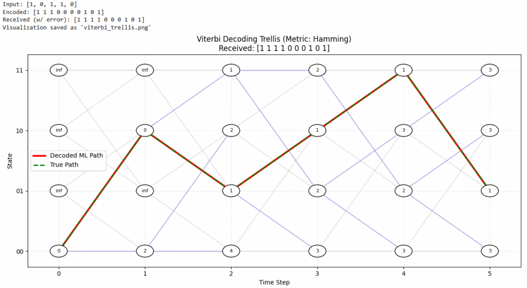
The Trellis Diagram
The operation of the encoder over time can be represented by a Trellis Diagram.
- Nodes: Represent states (00, 01, 10, 11) at discrete time steps $t$.
- Edges: Represent valid transitions between states triggered by an input bit (0 or 1).
- Labels: Each edge is labeled with the output symbol generated during that transition.
The problem of decoding is equivalent to finding the path through this trellis that matches the received sequence of bits most closely (minimizing the Hamming distance for hard decision decoding).
Viterbi Decoding and the ACS Block
The Viterbi algorithm efficiently explores the trellis to find the ML path. It does not test every single path (which grows exponentially); instead, it maintains the best path (survivor path) to each state at every time step.
Key Metrics
- Branch Metric (BM): The distance between the received symbol at time $t$ and the expected symbol for a specific edge.
- Hard Decision: Hamming distance (0, 1, or 2 bits different).
- Soft Decision: Euclidean distance or correlation metric.
- Path Metric (PM): The accumulated metric for a path up to the current state. $PM[state, t] = PM[prev_state, t-1] + BM$.
The ACS (Add-Compare-Select) Unit
The heart of the Viterbi decoder hardware/software is the ACS unit. For each state at time $t$:
- ADD: For every incoming branch (usually 2, one for input 0 and one for input 1), add the branch metric to the path metric of the previous state.
- $Candidate_0 = PM[State_{prev0}, t-1] + BM[Edge_{prev0 \to current}]$
- $Candidate_1 = PM[State_{prev1}, t-1] + BM[Edge_{prev1 \to current}]$
- COMPARE: Compare the candidate path metrics.
- Is $Candidate_0 < Candidate_1$? (Assuming we are minimizing distance).
- SELECT: Select the smaller metric as the new Path Metric for the current state.
- $PM[State_{current}, t] = \min(Candidate_0, Candidate_1)$
- Discard the other path. The edge corresponding to the winner is the Survivor Path. Store which previous state triggered this survivor (e.g., store a single bit “0” or “1”).
Traceback
Once the entire received sequence is processed (forward pass), we identify the state with the lowest final Path Metric. We then “trace back” through the stored decisions (survivor bits) to reconstruct the original input sequence.
The following is the visualization of a Viterbi decoder using Trellis diagram for a Rate 1/2, $K=3$ encoder
Hard Decision vs. Soft Decision Viterbi
The performance of the Viterbi decoder heavily depends on how the received analog signal is quantized before being processed by the decoder.
Hard Decision Viterbi
In Hard Decision decoding, the demodulator makes a firm decision on each received bit (0 or 1) before passing it to the Viterbi decoder.
- Input: Binary sequence (0s and 1s).
- Metric: Hamming Distance. The branch metric is simply the number of bit positions that differ between the received symbol and the expected symbol on the trellis edge.
- Pros/Cons: It is simpler to implement in hardware but results in a performance loss of approximately 2-3 dB compared to soft decision decoding because reliability information is discarded.
Soft Decision Viterbi
In Soft Decision decoding, the demodulator passes unquantized or finely quantized values (e.g., log-likelihood ratios or voltage levels) to the decoder.
- Input: Real numbers or multi-bit integers (e.g., 3-bit or 4-bit quantization) representing the confidence of the received bit.
- For example, a strong “1” might be +7, a weak “1” might be +1, a weak “0” might be -1, etc.
- Metric: Euclidean Distance (or Squared Euclidean Distance). The branch metric is $(r – v)^2$, where $r$ is the received soft value and $v$ is the expected symbol value (mapped to e.g., +1/-1). Alternatively, a correlation metric can be used.
- Pros/Cons: Soft decision decoding retains information about how certain the demodulator was about each bit. This typically yields a coding gain of about 2 dB over hard decision decoding in Gaussian noise. 3-bit quantization is often sufficient to achieve most of this gain.
Python Implementation: Hard-Decision Viterbi
This script demonstrates a simple Viterbi decoder for a Rate 1/2, $K=3$ convolutional code.
import numpy as np

def viterbi_decode(received_bits, trellis, num_states):
    """
    received_bits: List of bits received from the channel
    trellis: Dictionary defining transitions {state: {input_bit: (next_state, output_bits)}}
    """
    # Initialize path metrics with infinity
    path_metrics = {state: float('inf') for state in range(num_states)}
    path_metrics[0] = 0  # Start at state 0

    paths = {state: [] for state in range(num_states)}

    # Process received bits in pairs (Rate 1/2)
    for i in range(0, len(received_bits), 2):
        chunk = received_bits[i:i+2]
        new_metrics = {}
        new_paths = {}

        for state in range(num_states):
            for bit in [0, 1]:
                next_state, out = trellis[state][bit]

                # Calculate Hamming Distance (Branch Metric)
                branch_metric = sum(b1 != b2 for b1, b2 in zip(chunk, out))
                total_metric = path_metrics[state] + branch_metric

                if total_metric < new_metrics.get(next_state, float('inf')):
                    new_metrics[next_state] = total_metric
                    new_paths[next_state] = paths[state] + [bit]

        path_metrics = new_metrics
        paths = new_paths

    # Final selection: Path with the lowest metric
    best_state = min(path_metrics, key=path_metrics.get)
    return paths[best_state]

# Example Trellis for K=3, Rate 1/2 (G1=7, G2=5)
# Format: state: {input: (next_state, output)}
trellis_example = {
    0: {0: (0, [0,0]), 1: (2, [1,1])},
    1: {0: (0, [1,1]), 1: (2, [0,0])},
    2: {0: (1, [1,0]), 1: (3, [0,1])},
    3: {0: (1, [0,1]), 1: (3, [1,0])}
}

received = [1, 1, 0, 1, 1, 0] # Example received sequence
decoded = viterbi_decode(received, trellis_example, 4)
print(f"Decoded Bits: {decoded}")
Summary
Convolutional codes provide a powerful way to correct errors in communication channels by correlating bits over time. The Viterbi algorithm exploits this correlation using the ACS operation to efficiently prune unlikely paths through the trellis, ensuring that the final decoded sequence is the Maximum Likelihood estimate.
- Convolutional Encoding adds memory to the signal.
- The Trellis is a map of all possible “histories” of the signal.
- Viterbi Decoding is a “shortest path” algorithm that finds the most likely history.
- ACS is the engine that drives the decoding at every time step.