
Introduction
The Hamming codes described in previous articles are suitable for random bit errors. However, if the communication medium is prone to burst errors (contiguous blocks of bits being corrupted), Hamming codes are no longer efficient. For these scenarios, we use a class of Error Correcting Codes called Reed-Solomon (RS) Codes.
Applications of RS Codes
Reed-Solomon codes are useful for channels with “memory” (where errors occur in clusters). Common applications include:
- Storage Devices: CD, DVD, Blu-ray, and Hard Disk read/write channels.
- Broadband: Digital Subscriber Line (DSL), ADSL, and VDSL.
- Space & Wireless: Deep space/satellite communications and Digital Television (DVB).
- Barcodes: 2-dimensional barcodes like QR codes.
Symbols vs. Bits
RS codes are non-binary cyclic codes. While standard codes operate on bits, RS codes operate on symbols, which are groups of $m$ bits.
For example, if we use $m = 8$ bits per symbol, a single symbol error could mean 1 bit is wrong or all 8 bits in that symbol are wrong. From the perspective of the RS decoder, both cases count as only one symbol error. This is why RS codes are exceptionally good at handling burst errors.
Defining the (n, k) Parameters
An RS code is specified as an $(n, k)$ code with $m$-bit symbols.
- $n$ is the total number of symbols in the codeword: $n = 2^m – 1$
- $k$ is the number of data symbols.
- $n – k$ is the number of parity symbols (redundancy).
The length \(n = 2^m – 1\) is the full, primitive length. Codes that ship in products are often shortened: some information symbols are fixed at zero and never sent, and the receiver puts those zeros back before decoding. Shortening preserves the MDS distance \(d_{\min} = n – k + 1\) of the shorter word. The DVB-S outer code RS(204, 188) is a shortened RS(255, 239) over GF(256). QR codes use the same field at several shortened lengths.
The code can be defined by the following equation:
$$(n, k) = (2^m – 1, 2^m – 1 – 2t)$$
Where $t$ is the symbol error correcting capability.
Minimum Distance and Error Correction
The minimum distance for an RS code is given by:
$$d_{min} = n – k + 1 = 2t + 1$$
This provides the maximum possible $d_{min}$ for any linear code, making RS codes Maximum Distance Separable (MDS) codes. A higher $d_{min}$ means the code is more reliable and can correct more errors.
Example:
Consider a $(255, 247)$ RS code with $m = 8$ bits per symbol.
- $n = 255$ symbols
- $k = 247$ data symbols
- Parity symbols = $n – k = 8$
- Error capability $t = \frac{8}{2} = 4$ symbols.
This code corrects any pattern of 4 symbol errors, so it corrects a burst that stays inside 4 symbols. A burst that straddles a symbol boundary can touch one more symbol than the bit count suggests, and that extra symbol spends one unit of the budget \(t\). The same 8 parity symbols also correct erasures. If the decoder is told which \(\nu\) symbols were erased, and \(\varepsilon\) further symbols are wrong at unknown locations, correction succeeds whenever \(2\varepsilon + \nu \le n – k\).
Performance Effects
- Block length ($n$): At a fixed rate, a longer block makes the decoded error rate fall more steeply once the channel is better than the code’s threshold, and it costs latency and decoder work. Lengthening the block while holding the number of parity symbols fixed does the opposite: the rate rises and $t/n$ falls.
- Redundancy ($k$): As $k$ decreases (relative to $n$), the Code Rate ($R = k/n$) decreases, but the error-correcting capability increases.
- Optimum Code Rate: The design choice depends on the specific channel. The rate that requires the lowest $E_b/N_0$ for a target BER is considered the optimum.
Matlab Implementation
The following code simulates RS encoding and decoding. It demonstrates how the code succeeds when errors are within the capability $t$ and fails when they exceed it.
% Matlab Code for RS coding and decoding
n = 7; k = 3; % Codeword and message word lengths
m = 3;        % Number of bits per symbol (GF(2^3))

% Create message words over Galois Field
msg = gf([5 2 3; 0 1 7; 3 6 1], m);

% RS Encoding
codedMessage = rsenc(msg, n, k);
dmin = n - k + 1;
t = (dmin - 1) / 2; % Error correcting capability

% Generate noise:
% Row 1: 2 contiguous symbol errors (Should be corrected)
% Row 2: 2 discontiguous symbol errors (Should be corrected)
% Row 3: 3 distributed symbol errors (past t for this word; rsdec returns cnumerr = -1 here. Another pattern past t can be miscorrected)
noise = gf([0 0 0 2 3 0 0; 6 0 1 0 0 0 0; 5 0 6 0 0 4 0], m);
received = noise + codedMessage;

% RS Decoding
[dec, cnumerr] = rsdec(received, n, k);

% Display results
disp('Original Message:'); disp(msg);
disp('Decoded Message:'); disp(dec);
disp('Errors Corrected per row (-1 indicates failure):'); disp(cnumerr);
Analysis of Results
- Rows 1 & 2:
cnumerrreturns2. The errors are corrected because $2 \leq t$. - Row 3:
cnumerrreturns-1for this particular pattern. Three errors exceed \(t = 2\) of the $(7, 3)$ code, andrsdecdetects the failure. Do not read that as a promise for every pattern of three errors. A bounded-distance decoder can miscorrect a different pattern to the wrong codeword instead of returning-1.
Visualizing RS Code Performance
The performance of a Reed-Solomon code is often measured by plotting the decoded bit error probability (PB) against the raw channel symbol error probability (p).
To compute the Probability of Post-Decoding Bit Error ($P_B$) versus the Channel Symbol-Error Probability ($p$), we use the mathematical relationship defined by Bernard Sklar.
In an $(n,k)$ Reed-Solomon code that can correct up to t symbol errors, the probability that the decoder will fail or provide an incorrect symbol is the probability that more than t symbol errors occur in a block of n symbols.
Mathematical Formula
The probability of a decoded symbol being in error ($P_s$) is approximately:
$P_s \approx \frac{1}{n} \sum_{j=t+1}^{n}j\binom{n}{j}p^j\left(1-p \right)^{n-j}$
This is the expression used by Sklar. It treats a block with more than \(t\) errors as left unchanged, so the symbol errors that remain are exactly the ones the channel put there. A bounded-distance decoder does not always behave that way. Some patterns beyond \(t\) are detected as failures, and some are decoded to a wrong codeword, which adds further symbol errors. The formula is the right curve for a first comparison of code rates. It is an approximation once miscorrection is taken into account.
For an m-bit symbol, the relationship between the decoded symbol error probability ($P_s$) and the decoded bit error probability (PB) is:
$$\frac{P_B}{P_s} = \frac{2^{m-1}}{2^m-1}$$
Following Matlab code snippet and Python code helps to visualize the performance of different RS configurations.
Matlab
% Performance of Reed-Solomon Codes: PB vs Channel Symbol Error Probability (p)
% Reference: Bernard Sklar, "Reed-Solomon Codes"
% Mathuranathan Viswanathan @ gaussianwaves.com
clearvars; clc;

% --- Parameters ---
m = 8;               % Bits per symbol
n = 2^m - 1;         % Codeword length (255)
t_vec = [1, 2, 4, 8, 16]; % Error correcting capabilities requested
k_vec = n - 2*t_vec;      % Corresponding data lengths
p = logspace(-4, -1, 100); % Channel Symbol Error Probability (x-axis)

figure;
colors = {'#D95319', '#EDB120', '#7E2F8E', '#0072BD', '#A2142F'}; % Custom distinct colors

for idx = 1:length(t_vec)
    t = t_vec(idx);
    k = k_vec(idx);

    Ps_post = zeros(size(p));
    for i = 1:length(p)
        % Using binopdf for numerical stability with large n
        % We calculate the probability of more than t errors occurring
        j = (t+1):n;

        try
            % Requires Statistics and Machine Learning Toolbox
            prob_j_errors = binopdf(j, n, p(i));
        catch
            % Fallback for users without the toolbox
            prob_j_errors = arrayfun(@(x) exp(gammaln(n+1) - gammaln(x+1) - ...
                            gammaln(n-x+1)) .* (p(i)^x) .* ((1-p(i))^(n-x)), j);
        end

        % Sklar's formula for post-decoding symbol error probability
        Ps_post(i) = (1/n) * sum(j .* prob_j_errors);
    end

    % Convert Symbol Error Probability (Ps_post) to Bit Error Probability (PB)
    PB = Ps_post * (2^(m-1) / (2^m - 1));

    semilogy(p, PB, 'Color', colors{idx}, 'LineWidth', 2, ...
        'DisplayName', sprintf('RS(%d, %d), t=%d', n, k, t));
    hold on;
end

% --- Formatting to match Sklar's style ---
grid on;
set(gca, 'XDir', 'reverse'); % Reverse x-axis as per Sklar's convention
set(gca, 'XScale', 'log');
set(gca, 'YScale', 'log');
xlabel('Channel Symbol Error Probability (p)');
ylabel('Bit Error Probability (P_B)');
title('Reed-Solomon Code Performance (n=255, m=8)');
legend('Location', 'northeast');
axis([1e-4 1e-1 1e-15 1e-1]); % Adjusted Y-limits to show the deep waterfallPython
import numpy as np
import matplotlib.pyplot as plt
from scipy.stats import binom

# --- Parameters ---
m = 8                # Bits per symbol
n = 2**m - 1         # Codeword length (255)
t_vec = [1, 2, 4, 8, 16] # Error correcting capabilities
k_vec = [n - 2*t for t in t_vec] # Corresponding data lengths
p = np.logspace(-4, -1, 100)      # Channel Symbol Error Probability (x-axis)

# Conversion factor from Symbol Error Prob to Bit Error Prob
bit_err_factor = (2**(m-1)) / (2**m - 1)

plt.figure(figsize=(10, 7))

# --- Calculation and Plotting ---
for i, t in enumerate(t_vec):
    k = k_vec[i]
    pb_decoded = []

    for p_val in p:
        # Range of errors that exceed the capability t
        j = np.arange(t + 1, n + 1)

        # Probability of exactly j errors occurring in n symbols
        prob_j_errors = binom.pmf(j, n, p_val)

        # Sklar's formula for post-decoding symbol error probability:
        # Ps_post approx (1/n) * sum( j * Prob(j errors) )
        ps_post = (1/n) * np.sum(j * prob_j_errors)

        # Convert to Bit Error Probability (PB)
        pb_decoded.append(ps_post * bit_err_factor)

    plt.loglog(p, pb_decoded, label=f'RS({n}, {k}), t={t}', linewidth=2)

# --- Formatting to match Sklar's style ---
plt.gca().invert_xaxis() # Reverse x-axis: 10^-1 to 10^-4
plt.grid(True, which="both", linestyle='--', alpha=0.7)
plt.xlabel('Channel Symbol Error Probability (p)')
plt.ylabel('Bit Error Probability ($P_B$)')
plt.title(f'Reed-Solomon Code Performance (n={n}, m={m})')
plt.legend(loc='upper right')
plt.ylim(1e-15, 1e-1)
plt.xlim(1e-1, 1e-4)
plt.show()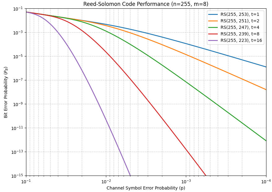
As seen in the generated plot, once the channel error rate drops below a certain “threshold,” the $P_B$ drops precipitously. This “waterfall” effect is characteristic of powerful block codes, showing how they can provide near-error-free communication even in noisy environments, provided the number of errors stays within the correction limit $t$.
Analyzing Error-Correcting Capability (t)
The plot illustrates how the error-correcting capability t impacts the reliability of the communication link.
- For $t=1$: The code provides a modest improvement. The “waterfall” is less steep, meaning the transition from a noisy to a clear channel is gradual.
- For $t=16$: The code is extremely powerful. Once the channel symbol error probability ($p$) drops below $10^{−2}$, the bit error rate PB drops instantly by several orders of magnitude.
This behavior highlights why Reed-Solomon codes are often described as having a “brick wall” performance characteristic—below a certain error threshold, the output is virtually error-free.
RS Codes and M-ary Modulation
When analyzing the performance of Reed-Solomon codes, it is common to pair them with M-ary modulation schemes where the modulation symbol size matches the code symbol size ($M = 2^m$). A classic example often cited is the RS(31, k) code using 32-ary MFSK modulation. This configuration is particularly efficient because a single channel symbol error translates exactly into a single Reed-Solomon symbol error. This one-to-one mapping avoids “error spreading,” where one corrupted channel symbol could potentially damage multiple code symbols, maximizing the efficiency of the decoder’s t-error correcting capability.
Following Matlab and Python scripts use the noncoherent M-ary orthogonal signaling formula and the parameters $n=31$,$m=5$ with $t=1,2,4,8$
Matlab
% RS(31, k) over Noncoherent 32-ary MFSK
% Author: Mathuranathan Viswanathan (www.gaussianwaves.com)
clearvars; clc;

% --- Parameters ---
m = 5; n = 31; M = 32;
t_vec = [1, 2, 4, 8];
EbN0_dB = 3:0.05:8;
EbN0_lin = 10.^(EbN0_dB/10);

figure('Color', 'w', 'Position', [100 100 650 800]);

for idx = 1:length(t_vec)
    t = t_vec(idx);
    k = n - 2*t;
    R = k/n;

    PB_rs = zeros(size(EbN0_lin));
    for i = 1:length(EbN0_lin)
        % 1. Channel Symbol Error Prob (p) for Noncoherent M-ary Orthogonal
        % Es/N0 = Eb/N0 * R * m
        EsN0 = EbN0_lin(i) * R * m;

        % Closed-form sum for noncoherent orthogonal M-FSK
        p = 0;
        for j = 1:(M-1)
            p = p + ((-1)^(j+1) / (j+1)) * nchoosek(M-1, j) * exp(-(j/(j+1)) * EsN0);
        end

        % 2. Post-Decoding Symbol Error Prob (Ps_post)
        % Using Sklar's Equation (7)
        errors = (t+1):n;
        prob_j = binopdf(errors, n, p);
        Ps_post = (1/n) * sum(errors .* prob_j);

        % 3. Bit Error Probability (PB) using Sklar's Equation (8)
        PB_rs(i) = Ps_post * (2^(m-1) / (2^m - 1));
    end

    semilogy(EbN0_dB, PB_rs, 'LineWidth', 2, 'DisplayName', sprintf('t = %d', t));
    hold on;
end

% Aesthetics to match PDF Figure 2
grid on;
xlabel('E_b/N_0 (dB)'); ylabel('Bit error probability, P_B');
title('RS(31, k) with 32-ary MFSK (Noncoherent)');
legend('Location', 'northeast');
axis([3.5 7 1e-7 1e-2]);Python
import numpy as np
import matplotlib.pyplot as plt
from scipy.special import comb
from scipy.stats import binom

# --- Parameters ---
m, n, M = 5, 31, 32
t_vec = [1, 2, 4, 8]
ebn0_db = np.arange(3.5, 7.1, 0.1)
ebn0_lin = 10**(ebn0_db / 10)

def noncoherent_mfsk_p(esn0, M):
    """Symbol error probability for noncoherent M-ary orthogonal signaling."""
    p = 0
    for j in range(1, M):
        term = ((-1)**(j+1) / (j+1)) * comb(M-1, j) * np.exp(-(j/(j+1)) * esn0)
        p += term
    return p

plt.figure(figsize=(7, 9))
bit_err_factor = (2**(m-1)) / (2**m - 1)

for t in t_vec:
    k = n - 2*t
    R = k/n
    pb_rs = []

    for en in ebn0_lin:
        # 1. Raw Channel Symbol Error
        p = noncoherent_mfsk_p(en * R * m, M)

        # 2. RS Decoding (Post-decoding symbol error)
        j_err = np.arange(t + 1, n + 1)
        prob_j = binom.pmf(j_err, n, p)
        ps_post = (1/n) * np.sum(j_err * prob_j)

        # 3. Final Bit Error
        pb_rs.append(ps_post * bit_err_factor)

    plt.semilogy(ebn0_db, pb_rs, label=f't = {t}', linewidth=2)

plt.grid(True, which='both', linestyle='-', alpha=0.5)
plt.xlabel('$E_b/N_0$ (dB)')
plt.ylabel('Bit error probability, $P_B$')
plt.xlim(3.5, 7.0)
plt.ylim(1e-7, 1e-2)
plt.legend()
plt.title("RS(31, k) with 32-ary MFSK Modulation")
plt.show()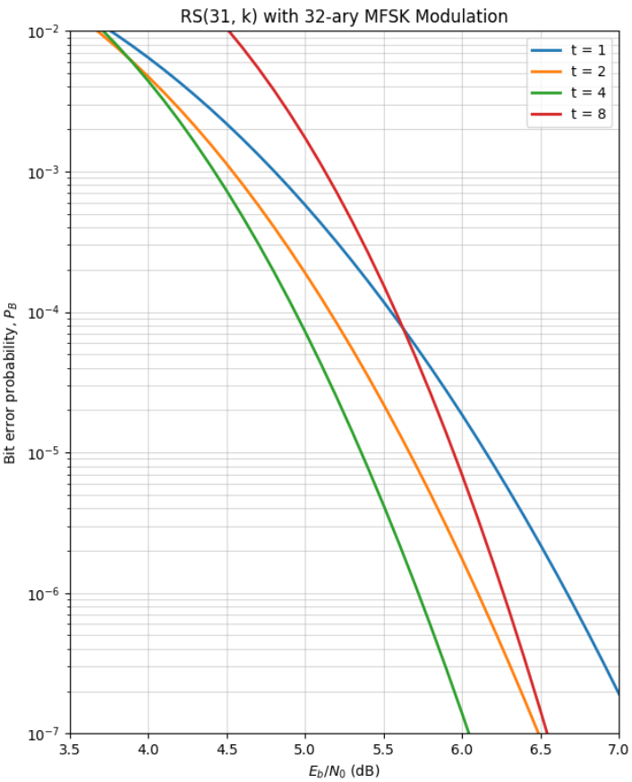
Solomon coding systems with $32$-ary MFSK modulation over an AWGN channel
Clearing the “MPSK vs. MFSK” Confusion
Students often encounter a famous contradiction in legacy literature—specifically in Bernard Sklar’s foundational work on Reed-Solomon codes. While some figure captions may inadvertently label the modulation as 32-ary MPSK, the performance curves tell a different story. If you look at the Eb/N0 scale, you’ll notice the “waterfall” performance begins as low as 4 to 6 dB. For 32-ary MPSK, such a low signal-to-noise ratio would result in an unusable link. The actual performance shown corresponds to Noncoherent M-ary Orthogonal signaling (MFSK), which is far more power-efficient than M-PSK in low-SNR environments, albeit at the cost of significantly higher bandwidth.
Analyzing the Threshold and “Cliff” Effect
The resulting BER curves illustrate the “brick wall” or “cliff” effect characteristic of block codes. Notice that at very low Eb/N0, a lower-rate code like t=8 might actually perform worse than a higher-rate t=1 code. This occurs because the parity overhead reduces the energy available for each information bit. However, once the channel quality crosses a specific threshold (the “knee” of the curve), the error-correcting power takes over, and the bit error probability PB drops by several orders of magnitude for just a fraction of a decibel increase in power. This trade-off between coding gain and bandwidth efficiency is the fundamental design choice in any RS-coded communication system.
References:
[1] Bernard Sklar, Mathematics behind RS codes.
[2] Introduction to Interleavers and Deinterleavers – GaussianWaves.