Derive BPSK BER – optimum receiver in AWGN channel

Key focus: Derive BPSK BER (bit error rate) for optimum receiver in AWGN channel. Explained intuitively step by step.

BPSK modulation is the simplest of all the M-PSK techniques. An insight into the derivation of error rate performance of an optimum BPSK receiver is essential as it serves as a stepping stone to understand the derivation for other comparatively complex techniques like QPSK,8-PSK etc..

Understanding the concept of Q function and error function is a pre-requisite for this section of article.

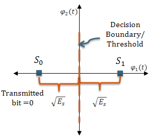
The ideal constellation diagram of a BPSK transmission (Figure 1) contains two constellation points located equidistant from the origin. Each constellation point is located at a distance from the origin, where E_s is the BPSK symbol energy. Since the number of bits in a BPSK symbol is always one, the notations – symbol energy (E_s) and bit energy (E_b) can be used interchangeably (E_s=E_b).

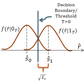
Assume that the BPSK symbols are transmitted through an AWGN channel characterized by variance = N₀/2 Watts. When 0 is transmitted, the received symbol is represented by a Gaussian random variable ‘r‘ with mean=S₀ = and variance =N₀/2. When 1 is transmitted, the received symbol is represented by a Gaussian random variable – r with mean=S₁= and variance =N₀/2. Hence the conditional density function of the BPSK symbol (Figure 2) is given by,

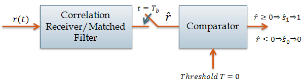
 An optimum receiver for BPSK can be implemented using a correlation receiver or a matched filter receiver (Figure 3). Both these forms of implementations contain a decision making block that decides upon the bit/symbol that was transmitted based on the observed bits/symbols at its input.

When the BPSK symbols are transmitted over an AWGN channel, the symbols appears smeared/distorted in the constellation depending on the SNR condition of the channel. A matched filter or that was previously used to construct the BPSK symbols at the transmitter. This process of projection is illustrated in Figure 4. Since the assumed channel is of Gaussian nature, the continuous density function of the projected bits will follow a Gaussian distribution. This is illustrated in Figure 5.

After the signal points are projected on the basis function axis, a decision maker/comparator acts on those projected bits and decides on the fate of those bits based on the threshold set. For a BPSK receiver, if the a-prior probabilities of transmitted 0’s and 1’s are equal (P=0.5), then the decision boundary or threshold will pass through the origin. If the apriori probabilities are not equal, then the optimum threshold boundary will shift away from the origin.

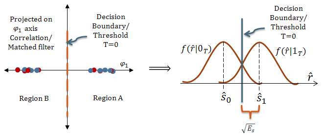
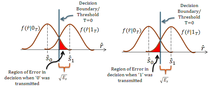
Considering a binary symmetric channel, where the apriori probabilities of 0’s and 1’s are equal, the decision threshold can be conveniently set to T=0. The comparator, decides whether the projected symbols are falling in region A or region B (see Figure 4). If the symbols fall in region A, then it will decide that 1 was transmitted. It they fall in region B, the decision will be in favor of ‘0’.

For deriving the performance of the receiver, the decision process made by the comparator is applied to the underlying distribution model (Figure 5). The symbols projected on the axis will follow a Gaussian distribution. The threshold for decision is set to T=0. A received bit is in error, if the transmitted bit is ‘0’ & the decision output is ‘1’ and if the transmitted bit is ‘1’ & the decision output is ‘0’.

This is expressed in terms of probability of error as,

Or equivalently,

By applying Bayes Theorem↗, the above equation is expressed in terms of conditional probabilities as given below,

Since a-prior probabilities are equal P(0_T)= P(1_T) =0.5, the equation can be re-written as

Intuitively, the integrals represent the area of shaded curves as shown in Figure 6. From the previous article, we know that the area of the shaded region is given by Q function.

Similarly,

From (4), (6), (7) and (8),

For BPSK, since E_s=E_b, the probability of symbol error (P_s) and the probability of bit error (P_b) are same. Therefore, expressing the P_s and P_b in terms of Q function and also in terms of complementary error function :

Rate this article: (19 votes, average: 4.37 out of 5)

Reference

[1] Nguyen & Shwedyk, “A First course in Digital Communications”, Cambridge University Press, 1st edition.↗

Books by author

Wireless Communication Systems in Matlab Second Edition(PDF) (180 votes, average: 3.62 out of 5) $14.99 – Add to Cart Checkout Added to cart	Digital Modulations using Python (PDF ebook) (134 votes, average: 3.56 out of 5) $14.99 – Add to Cart Checkout Added to cart	Digital Modulations using Matlab (PDF ebook) (136 votes, average: 3.63 out of 5) $14.99 – Add to Cart Checkout Added to cart
Hand-picked Best books on Communication Engineering Best books on Signal Processing