Ergodic Capacity of SISO flat fading channel

Understand ergodic capacity of a SISO flat-fading system over fading channels. Model and simulate capacity curves in Matlab.

Channel model

In the previous post, derivation of SISO fading channel capacity was discussed. For a flat fading channel (model shown below), with the perfect knowledge of the channel at the receiver, the capacity of a SISO link was derived as

$latex C = log_2 (1 + \gamma)=log_2 \left ( 1 + \frac{P_t}{\sigma_n^2} \left | h \right |^2 \right ) \quad \quad\quad (1) &s=2$

where,  $latex h$ is flat fading complex channel impulse response that is held constant for each block of $latex N$ transmitted symbols, $latex P_t$ is the average input power at the transmit antenna, $latex \gamma = \frac{P_t}{\sigma_n^2} \left | h \right |^2 $ is the signal-to-noise ratio (SNR) at the receiver input and $latex \sigma_n^2$ is the noise power of the channel.

Since the channel impulse response $latex h$ is a random variable, the channel capacity equation shown above is also random. To circumvent this, Ergodic channel capacity was defined along with outage capacity. The Ergodic channel capacity is defined as the statistical average of the mutual information, where the expectation is taken over $latex \left | h \right |^2 $

$latex C_{erg}=\mathbb{E} \left\{ log_2 \left ( 1 + \frac{P_t}{\sigma_n^2} \left | h \right |^2 \right ) \right\}  \quad \quad \quad (2) &s=2$

Jensen’s inequality [1] states that for any concave function f(x), where x is a random variable,

$latex E[f(X)] \leq f(E[X]) \quad\quad (3) &s=2$

Applying Jensen’s inequality to Ergodic capacity in equation (2),

$latex \mathbb{E} \left[ log_2 \left ( 1 + \frac{P_t}{\sigma_n^2} \left | h \right |^2 \right ) \right] \leq log_2 \left ( 1 + \frac{P_t}{\sigma_n^2}  \mathbb{E} [\left | h \right |^2] \right ) \quad\quad (4) &s=2$

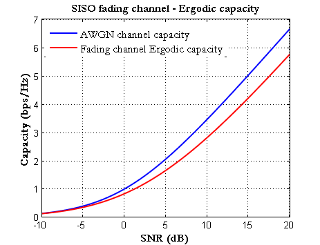
This implies that the Ergodic capacity of a fading channel cannot exceed that of an AWGN channel with constant gain. The above equation is simulated in Matlab for a Rayleigh Fading channel with $latex \sigma_h^2=E |h|^2=1 , \sigma_n^2=1$and the plots are shown below.

Matlab code

%This work is licensed under a Creative Commons
%Attribution-NonCommercial-ShareAlike 4.0 International License
%Attribute author : Mathuranathan Viswanathan at gaussianwaves.com
snrdB=-10:0.5:20; %Range of SNRs to simulate

h= (randn(1,100) + 1i*randn(1,100) )/sqrt(2); %Rayleigh flat channel
sigma_z=1; %Noise power - assumed to be unity


snr = 10.^(snrdB/10); %SNRs in linear scale
P=(sigma_z^2)*snr./(mean(abs(h).^2)); %Calculate corresponding values for P

C_erg_awgn= (log2(1+ mean(abs(h).^2).*P/(sigma_z^2))); %AWGN channel capacity (Bound)
C_erg = mean((log2(1+ ((abs(h).^2).')*P/(sigma_z^2)))); %ergodic capacity for Fading channel

plot(snrdB,C_erg_awgn,'b'); hold on;
plot(snrdB,C_erg,'r'); grid on;
legend('AWGN channel capacity','Fading channel Ergodic capacity');
title('SISO fading channel - Ergodic capacity');
xlabel('SNR (dB)');ylabel('Capacity (bps/Hz)');

Rate this article: [ratings]

References

[1] Konstantinos G. Derpanis, Jensen’s Inequality, Version 1.0,March 12, 2005.↗

[table id=17 /]

Books by the author

[table id=23 /]