Key focus: Shown with examples: let’s estimate and plot the probability density function of a random variable using Python’s Matplotlib histogram function.
This post contains interactive python code which you can execute in the browser itself.
Generation of random variables with required probability distribution characteristic is of paramount importance in simulating a communication system. Let’s see how we can generate a simple random variable, estimate and plot the probability density function (PDF) from the generated data and then match it with the intended theoretical PDF. Normal random variable is considered here for illustration.
Step 1: Generate random samples
A survey of commonly used fundamental methods to generate a given random variable is given in [1]. For this demonstration, we will consider the normal random variable with the following parameters : μ – mean and σ – standard deviation. First generate a vector of randomly distributed random numbers of sufficient length (say 100000) with some valid values for μ and σ. There are more than one way to generate this. Two of them are given below.
● Method 1: Using the in-built numpy.random.normal() function (requires numpy package to be installed)
import numpy as np

mu=10;sigma=2.5 #mean=10,deviation=2.5
L=100000 #length of the random vector

#Random samples generated using numpy.random.normal()
samples_normal = np.random.normal(loc=mu,scale=sigma,size=(L,1)) #generate normally distributted samples
● Method 2: Box-Muller transformation [2] method produces a pair of normally distributed random numbers (Z1, Z2) by transforming a pair of uniformly distributed independent random samples (U1,U2). The algorithm for transformation is given by

#Samples generated using Box-Muller transformation

U1 = np.random.uniform(low=0,high=1,size=(L,1)) #uniformly distributed random numbers U(0,1)
U2 = np.random.uniform(low=0,high=1,size=(L,1)) #uniformly distributed random numbers U(0,1)

a = np.sqrt(-2*np.log(U1))
b = 2*np.pi*U2

Z = a*np.cos(b) #Standard Normal distributed numbers
samples_box_muller= Z*sigma+mu #Normal distribution with mean and sigma
Step 2: Plot the estimated histogram
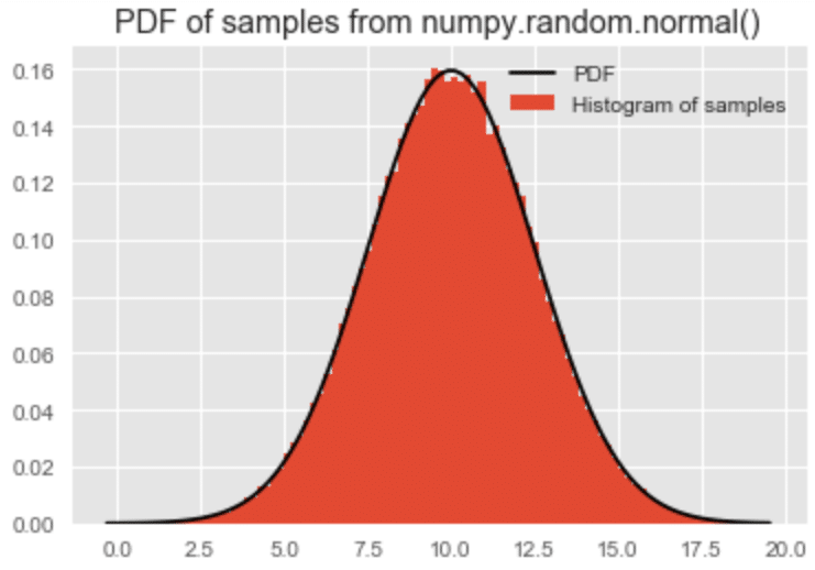
Typically, if we have a vector of random numbers that is drawn from a distribution, we can estimate the PDF using the histogram tool. Matplotlib’s hist function can be used to compute and plot histograms. If the density argument is set to ‘True’, the hist function computes the normalized histogram such that the area under the histogram will sum to 1. Estimate and plot the normalized histogram using the hist function.
#For plotting
import matplotlib.pyplot as plt
import matplotlib

# matplotlib backend needed with inseri-core
matplotlib.use('Agg')

plt.style.use('ggplot')

fig, ax0 = plt.subplots(ncols=1, nrows=1) #creating plot axes
(values, bins, _) = ax0.hist(samples_normal,bins=100,density=True,label="Histogram of samples") #Compute and plot histogram, return the computed values and bins
Step 3: Theoretical PDF:
And for verification, overlay the theoretical PDF for the intended distribution. The theoretical PDF of normally distributed random samples is given by

Theoretical PDF for normal distribution is readily obtained from stats.norm.pdf() function in the SciPy package.
from scipy import stats
bin_centers = 0.5*(bins[1:] + bins[:-1])
pdf = stats.norm.pdf(x = bin_centers, loc=mu, scale=sigma) #Compute probability density function
ax0.plot(bin_centers, pdf, label="PDF",color='black') #Plot PDF
ax0.legend()#Legend entries
ax0.set_title('PDF of samples from numpy.random.normal()');

plt.savefig("img.png", format='png', bbox_inches='tight')
plt.close()
plt.show()
Interactive Code:
Run the following interactive code to see the results below
Simulation result:
Reference result:

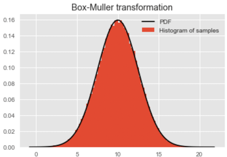
The histogram and theoretical PDF of random samples generated using Box-Muller transformation, can be plotted in a similar manner.
#Samples generated using Box-Muller transformation
from numpy.random import uniform
U1 = uniform(low=0,high=1,size=(L,1)) #uniformly distributed random numbers U(0,1)
U2 = uniform(low=0,high=1,size=(L,1)) #uniformly distributed random numbers U(0,1)
a = np.sqrt(-2*np.log(U1))
b = 2*np.pi*U2
Z = a*np.cos(b) #Standard Normal distribution
samples_box_muller = Z*sigma+mu #Normal distribution with mean and sigma

#Plotting
fig, ax1 = plt.subplots(ncols=1, nrows=1) #creating plot axes
(values, bins, _) = ax1.hist(samples_box_muller,bins=100,density=True,label="Histogram of samples") #Plot histogram
bin_centers = 0.5*(bins[1:] + bins[:-1])
pdf = stats.norm.pdf(x = bin_centers, loc=mu, scale=sigma) #Compute probability density function
ax1.plot(bin_centers, pdf, label="PDF",color='black') #Plot PDF
ax1.legend()#Legend entries
ax1.set_title('Box-Muller transformation');

References:
[1] John Mount, ‘Six Fundamental Methods to Generate a Random Variable’, January 20, 2012
[2] Thomas, D. B., Luk. W., Leong, P. H. W., and Villasenor, J. D. 2007. Gaussian random number generators. ACM Comput. Surv. 39, 4, Article 11 (October 2007), 38 pages DOI = 10.1145/1287620.1287622 http://doi.acm.org/10.1145/1287620.1287622
Rate this post: [ratings]
