
Articles in this series
- Phased array antenna — an introduction (this article)
- Electronic scanning arrays
- Grating lobes in electronic scanning
- Array pattern multiplication
Introduction
Suppose you need a radar beam that jumps from one track to another in a few microseconds, or a base-station panel that must serve users across a sector without swinging a dish. Mechanical rotation is too slow for that. A phased array points by arithmetic: many small antennas, each fed with a chosen amplitude and phase, so the fields add in one direction and cancel in others.
We will build that idea in four steps. This note covers architecture and the basic vocabulary. Next come electronic scanning on a uniform linear array, grating lobes as spatial aliases, and finally the product of array factor, element pattern, and amplitude taper. Hold those four pictures and you can read most AESA descriptions without getting lost.
Motive
Why bother? Because 5G panels, satellite terminals, and automotive radar are already arrays, whether or not the brochure says “MIMO.” Beams and nulls are set by the complex weights \(a_n e^{j\psi_n}\). Once those weights feel like ordinary control knobs, the later formulas are easier to follow.
Technical development
What is being controlled?
In the far field, shifting an element by \(\mathbf{l}_n\) multiplies its contribution by \(e^{j\mathbf{k}\cdot\mathbf{l}_n}\). If the feed applies the conjugate progressive phase, that geometric phase cancels in one look direction—and the beam points there. The amplitudes \(a_n\) set the illumination: sidelobes versus beamwidth versus aperture efficiency.
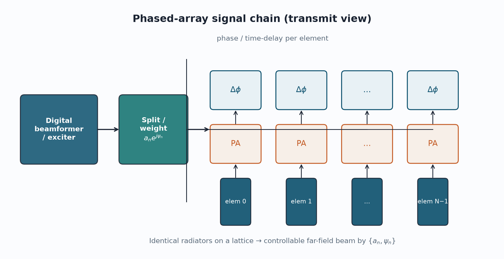
Phase shift versus true time delay
Narrowband arrays often use digital phase shifters (4–6 bits are common). Over a wide fractional bandwidth a pure phase command makes the beam squint with frequency; true time delay avoids that. For the classroom work ahead we stay narrowband: one frequency, one progressive phase.
How this achieves the motive
Look at Figure 1. Give every element a complex weight and you can steer by changing phases, shape sidelobes with an amplitude table, and form several beams by applying several weight vectors to the same aperture samples. The electromagnetics did not change; only how we set the weights did.
Sample simulation
Before the full derivation, try this small uniform linear array (ULA) factor. It is the same kernel we use later. Here \(u=\sin\theta\), spacing is \(d=\lambda/2\), and eight elements sit broadside.
import numpy as np
import matplotlib.pyplot as plt

def array_factor(u, N, d_over_lambda, u0=0.0):
    kdl = 2 * np.pi * d_over_lambda
    af = sum(np.exp(1j * n * kdl * (u - u0)) for n in range(N))
    g = np.abs(af) ** 2
    return g / np.max(g)

u = np.linspace(-1, 1, 2001)
g = array_factor(u, N=8, d_over_lambda=0.5, u0=0.0)
plt.plot(u, 10 * np.log10(np.maximum(g, 1e-6)))
plt.xlabel("u = sin(theta)"); plt.ylabel("|AF|^2 (dB)")
plt.grid(True); plt.show()
Sample results
You should see a main beam at \(u=0\) and sidelobes falling away—the usual Dirichlet-kernel shape of a uniform array. Increase \(N\) and the beam narrows. Set a nonzero \(u_0\) and the beam steers; that is the next article.
Next topic
Next we put phase shifters on paper and work out electronic scanning: path delay, progressive phase, and the closed-form array factor.
References
[1] C. A. Balanis, Antenna Theory. [2] R. J. Mailloux, Phased Array Antenna Handbook. [3] S. J. Orfanidis, Electromagnetic Waves and Antennas.