ENBW of FFT windows — formula, table, Matlab & Python

FFT measurement path:
Spectral leakage → ENBW of windows → Window figures of merit → Interpreting FFT bins

Interactive demo: FFT window functions — compare time/frequency shapes, ENBW, scalloping, and sidelobes in the browser.

In one sentence: ENBW tells how much white noise a FFT window passes — use it to correct noise-floor and PSD estimates.

Matlab/Python simulation: Compute ENBW from window samples, compare to the table, and explore shapes in the window functions demo.

Searchers looking for “equivalent noise bandwidth” usually want three things: the definition, the time-domain formula used in code, and a table of ENBW (in FFT bins) for common SciPy/Matlab windows. This page covers all three.

Why FFT bins are not brick walls

A length-$latex N$ DFT can be viewed as a bank of filters, each centered on a bin with nominal spacing $latex \Delta f = f_s/N$. In the ideal textbook picture those filters are narrow rectangles. Real signals are time-limited, so the FFT implicitly periodizes the observed slice. Edge discontinuities spill energy across bins — spectral leakage.

DFT viewed as a set of filter banks — *Figure 1: DFT viewed as processing through a set of filter banks.*

Multiplying by a window softens the edges and reduces leakage, but it also widens each bin’s effective noise bandwidth. The noise floor you read from an FFT therefore depends on the window — unless you correct by ENBW.

Definition of ENBW

Let $latex W(f)$ be the Fourier transform of the window. The noise power collected by the window is

\[P_{\mathrm{window}} = \int |W(f)|^2\,df\]

ENBW $latex B_{\mathrm{enbw}}$ is the bandwidth of a brick-wall filter with the same peak gain that collects the same noise power:

\[B_{\mathrm{enbw}}\,|W(f_0)|^2 = P_{\mathrm{window}} \quad\Rightarrow\quad B_{\mathrm{enbw}} = \frac{\int |W(f)|^2\,df}{|W(f_0)|^2}\]

Illustrating equivalent noise bandwidth versus a brick-wall filter — *Figure 2: ENBW as the brick-wall width that matches window noise power (not to scale).*

With DFT samples, and using Parseval’s relation on a length-$latex L$ window $latex w[n]$, the usual bins form is

\[B_{\mathrm{enbw}} = L\,\frac{\sum_n |w[n]|^2}{\left|\sum_n w[n]\right|^2}\]

That is the quantity SciPy’s signal.windows and Matlab’s enbw report. The noise-floor correction in dB is simply $latex 10\log_{10}(B_{\mathrm{enbw}})$.

*Figure 3: ENBW illustrated for a Hann window.*

ENBW of common windows (bins)

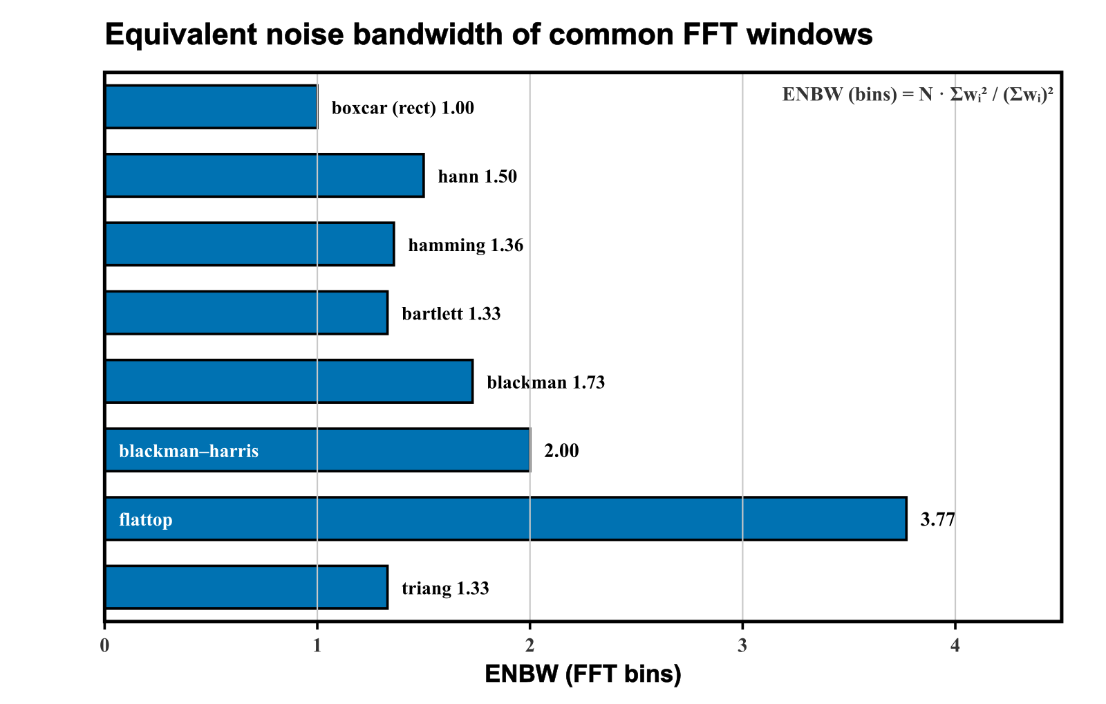
Figure 4 ranks several everyday windows. Rectangular (boxcar) sits at 1.00 bin by definition; Hann ≈ 1.50; Blackman–Harris ≈ 2.00; flattop is much wider (~3.77) because it optimizes amplitude flatness, not noise bandwidth.

Bar chart of equivalent noise bandwidth in FFT bins for common windows — Figure 4: ENBW (FFT bins) for common windows. Values from $latex L\sum w_i^2/(\sum w_i)^2$ with large $latex L$.

Python: compute ENBW for SciPy windows

Modern SciPy exposes windows under scipy.signal.windows. Avoid the deprecated DataFrame.append; build rows and construct the frame once.

import numpy as np
import pandas as pd
from scipy.signal import windows

def enbw(w):
    """Equivalent noise bandwidth in FFT bins."""
    w = np.asarray(w, dtype=float)
    return len(w) * np.sum(w**2) / (np.sum(w) ** 2)

names = [
    "boxcar", "barthann", "bartlett", "blackman", "blackmanharris",
    "bohman", "cosine", "flattop", "hamming", "hann", "nuttall",
    "parzen", "triang",
]
L = 16384
rows = []
for name in names:
    w = getattr(windows, name)(L)
    b = enbw(w)
    rows.append({
        "Window": name,
        "ENBW (bins)": round(b, 3),
        "ENBW correction (dB)": round(10 * np.log10(b), 3),
    })
df = pd.DataFrame(rows)
print(df.to_string(index=False))

Example output (rounded) matches Figure 4: boxcar 1.000 (0 dB), hann ≈ 1.500 (~1.76 dB), flattop ≈ 3.77 (~5.76 dB).

Table of ENBW for common window functions — *Table 1: ENBW and dB correction for common windows.*

What ENBW does to the noise floor

Figure 5 compares FFT spectra of the same noisy tone through boxcar vs flattop. The tone amplitude can look similar (especially with flattop’s flat main lobe), but the noise floor rises with ENBW. Subtract $latex 10\log_{10}(B_{\mathrm{enbw}})$ when you want window-independent noise density.

Noise floor comparison: flattop vs boxcar window FFT — *Figure 5: Noise floor vs ENBW — flattop vs boxcar on a noisy 10 Hz tone (Fs = 160 Hz, L = 2048, SNR = 30 dB).*

FAQ

Is ENBW the same as resolution bandwidth (RBW)? They are related but not identical. RBW is often taken from the −3 dB main-lobe width of the window’s frequency response, while ENBW is defined from noise power: how wide a brick-wall filter would need to be to pass the same noise power as the windowed FFT bin. For a rectangular window both equal one bin; for tapered windows ENBW is usually larger than the −3 dB width.

When should I apply the ENBW dB correction? Use it when you compare noise floors or noise spectral density across different windows (or against a rectangular reference). Tone-peak amplitude measurements use a different correction — coherent gain / processing gain — because a sinusoid adds coherently across the window while noise adds in power.

Can I see ENBW interactively? Yes — the FFT window functions demo plots each window and reports ENBW in bins and dB. For the comparison tables and scalloping discussion, continue with window figures of merit.

Reference

[1] Stefan Scholl, “Exact Signal Measurements using FFT Analysis,” Microelectronic Systems Design Research Group, TU Kaiserslautern — PDF.