BPSK Bit Error Rate in AWGN: Derivation and Simulation

The BPSK bit error rate for an optimum receiver in AWGN follows from a simple decision-threshold argument. This post derives it step by step, then checks the result with a Monte Carlo simulation in Python and Matlab.

System model

BPSK maps each bit to one of two antipodal symbols on the real line. Bit 0 maps to $s_0 = +\sqrt{E_s}$ and bit 1 maps to $s_1 = -\sqrt{E_s}$. Since one BPSK symbol carries one bit, $E_s = E_b$.

The channel adds white Gaussian noise with variance $N_0/2$ per real dimension. After the correlator or matched filter projects the received signal onto the basis function, the sample is

$$r = s_i + n, \qquad n \sim \mathcal{N}(0, N_0/2)$$

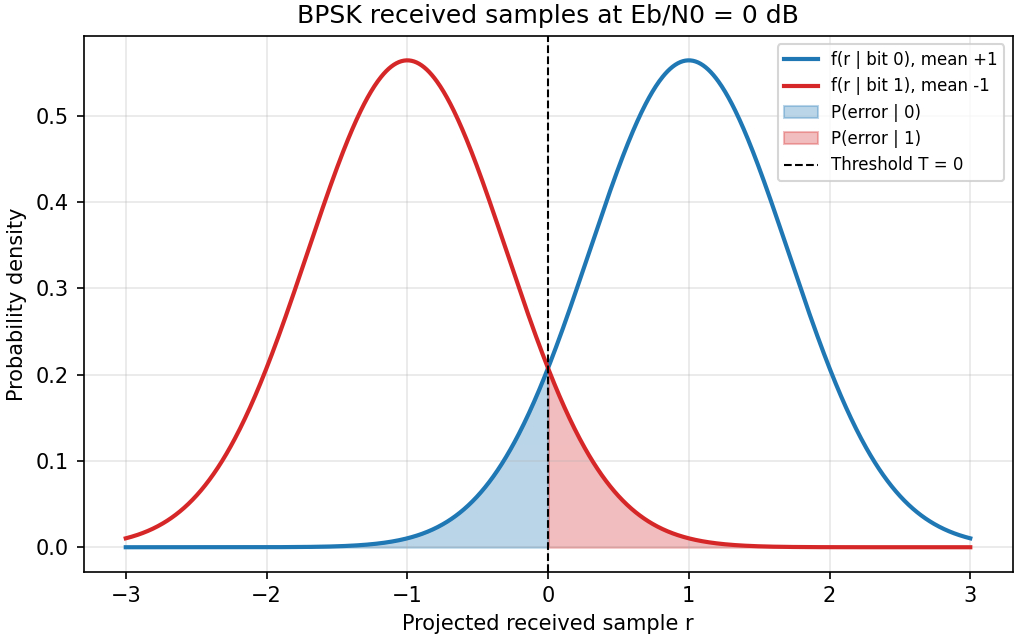
Given that bit 0 was sent, $r$ is Gaussian with mean $+\sqrt{E_s}$ and variance $N_0/2$. Given that bit 1 was sent, $r$ has mean $-\sqrt{E_s}$ and the same variance. The conditional densities are

$$f(r \mid 0) = \frac{1}{\sqrt{\pi N_0}} \exp\left(-\frac{(r – \sqrt{E_s})^2}{N_0}\right)$$

$$f(r \mid 1) = \frac{1}{\sqrt{\pi N_0}} \exp\left(-\frac{(r + \sqrt{E_s})^2}{N_0}\right)$$

The optimum decision rule compares $r$ with a threshold. When the two bits are equally likely, the threshold is $T = 0$. The receiver decides bit 0 when $r > 0$ and bit 1 when $r < 0$. If the bits are not equally likely, the optimum threshold moves away from the origin.

Deriving the error probability

With equal priors, the probability of error is the average of the two conditional error probabilities:

$$P_e = \tfrac{1}{2}\, P(r < 0 \mid 0) + \tfrac{1}{2}\, P(r > 0 \mid 1)$$

By symmetry the two terms are equal. Consider the first. Given bit 0, $r$ has mean $\sqrt{E_s}$ and standard deviation $\sqrt{N_0/2}$. Standardizing gives

$$P(r < 0 \mid 0) = P\left(Z < -\frac{\sqrt{E_s}}{\sqrt{N_0/2}}\right) = Q\left(\sqrt{\frac{2E_s}{N_0}}\right)$$

where $Q(x) = P(Z > x)$ is the Gaussian tail function. Since $E_s = E_b$ for BPSK, the symbol error rate and the bit error rate are equal:

$$P_s = P_b = Q\left(\sqrt{\frac{2E_b}{N_0}}\right) = \frac{1}{2}\,\mathrm{erfc}\left(\sqrt{\frac{E_b}{N_0}}\right)$$

The second form uses the identity $Q(\sqrt{2x}) = \tfrac{1}{2}\,\mathrm{erfc}(\sqrt{x})$. Both forms are standard, and the Q-function article lists the conversion.

Simulation in Python

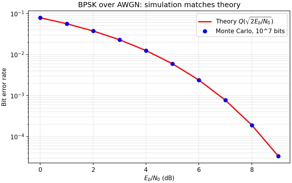
The simulation sends $10^7$ random bits through the AWGN model at each $E_b/N_0$ from 0 to 9 dB and counts the errors. The theory curve is $Q(\sqrt{2E_b/N_0})$.

import numpy as np
from scipy.special import erfc


def q_func(x):
    """Gaussian tail probability Q(x)."""
    return 0.5 * erfc(x / np.sqrt(2))


rng = np.random.default_rng(1)
n_bits = 10_000_000
bits = rng.integers(0, 2, n_bits)
s = 1.0 - 2.0 * bits                  # bit 0 -> +1, bit 1 -> -1, with Es = Eb = 1

for ebn0_db in range(10):
    ebn0 = 10 ** (ebn0_db / 10)
    n0 = 1 / ebn0                     # Es = 1, so N0 = Es / (Eb/N0)
    r = s + rng.normal(0, np.sqrt(n0 / 2), n_bits)
    bits_hat = (r < 0).astype(int)    # threshold T = 0
    ber_sim = np.mean(bits_hat != bits)
    ber_theory = q_func(np.sqrt(2 * ebn0))
    print(f"{ebn0_db} dB  sim={ber_sim:.3e}  theory={ber_theory:.3e}")

import numpy as np
from scipy.special import erfc


def q_func(x):
    """Gaussian tail probability Q(x)."""
    return 0.5 * erfc(x / np.sqrt(2))


rng = np.random.default_rng(1)
n_bits = 10_000_000
bits = rng.integers(0, 2, n_bits)
s = 1.0 - 2.0 * bits                  # bit 0 -> +1, bit 1 -> -1, with Es = Eb = 1

for ebn0_db in range(10):
    ebn0 = 10 ** (ebn0_db / 10)
    n0 = 1 / ebn0                     # Es = 1, so N0 = Es / (Eb/N0)
    r = s + rng.normal(0, np.sqrt(n0 / 2), n_bits)
    bits_hat = (r < 0).astype(int)    # threshold T = 0
    ber_sim = np.mean(bits_hat != bits)
    ber_theory = q_func(np.sqrt(2 * ebn0))
    print(f"{ebn0_db} dB  sim={ber_sim:.3e}  theory={ber_theory:.3e}")

Simulation in Matlab

The Matlab version uses the same model and the built-in erfc for the theory curve.

rng(1);
nBits = 1e7;
ebn0dB = 0:9;
bits = randi([0 1], nBits, 1);
s = 1 - 2*bits;                      % bit 0 -> +1, bit 1 -> -1 (Es = Eb = 1)
for k = 1:numel(ebn0dB)
    ebn0 = 10^(ebn0dB(k)/10);
    n0 = 1/ebn0;
    r = s + sqrt(n0/2)*randn(nBits, 1);
    bitsHat = double(r < 0);
    berSim = mean(bitsHat ~= bits);
    berTheory = 0.5*erfc(sqrt(ebn0));
    fprintf('%d dB  sim=%.3e  theory=%.3e\n', ebn0dB(k), berSim, berTheory);
end

rng(1);
nBits = 1e7;
ebn0dB = 0:9;
bits = randi([0 1], nBits, 1);
s = 1 - 2*bits;                      % bit 0 -> +1, bit 1 -> -1 (Es = Eb = 1)
for k = 1:numel(ebn0dB)
    ebn0 = 10^(ebn0dB(k)/10);
    n0 = 1/ebn0;
    r = s + sqrt(n0/2)*randn(nBits, 1);
    bitsHat = double(r < 0);
    berSim = mean(bitsHat ~= bits);
    berTheory = 0.5*erfc(sqrt(ebn0));
    fprintf('%d dB  sim=%.3e  theory=%.3e\n', ebn0dB(k), berSim, berTheory);
end

The Python and Matlab runs use different random generators, so their error counts differ slightly. Both match theory within the statistical noise.

Table 1: Python results with default_rng(1) and $10^7$ bits. The simulation agrees with theory to within about 1 percent at these points.

Summary

For BPSK over AWGN with an optimum receiver and equal priors, the bit error rate is $Q(\sqrt{2E_b/N_0})$. The derivation needs only the symbol mapping, the noise variance $N_0/2$, and the threshold at zero. The Monte Carlo results confirm it.

References

[1] Nguyen and Shwedyk, “A First Course in Digital Communications”, Cambridge University Press, 2009. https://doi.org/10.1017/cbo9780511841583

FAQs

Does the Q-function result match simulation? Yes — for coherent BPSK in AWGN the theoretical BER is $Q(\sqrt{2E_b/N_0})$. Compare your Monte Carlo curve to theory with the BER calculator and the dual-language sim: BPSK BER in Python & Matlab.

What breaks the “optimum receiver” assumption? Phase errors, imperfect timing, fading, and interference. Start from the AWGN derivation here, then move to fading/BER articles once the AWGN baseline matches theory.

Related: Eb/N0 ↔ Es/N0 ↔ SNR conversions for BER simulations (with Python).