Phased array series: 1. Introduction → 2. Electronic scanning → 3. Grating lobes (you are here) → 4. Array pattern multiplication
In one sentence: a grating lobe is an extra copy of the main beam. It appears when the elements are spaced too far apart, and it can point power in a direction you never wanted.
In the last article we steered a beam by putting a phase ramp across the elements. Then I got greedy. If elements can be spaced farther apart, the array gets smaller and cheaper, so why not? That is where the trap is. In this article I’ll show you where grating lobes come from, draw the one inequality you need to avoid them, and check it with a few numbers.
Why an array can have more than one main beam: grating lobes
Take $N$ identical isotropic elements in a line, spaced $d$ apart, all with equal weight. Let $u = sintheta$. The array factor is
$$AF(u) = sum_{n=0}^{N-1} e^{,j 2pi frac{d}{lambda}, n,(u – u_0)}.$$
Each term is a phase ramp. Between neighbouring elements the phase changes by $2pi (d/lambda)(u – u_0)$. The sum adds up in phase whenever that step is a whole multiple of $2pi$. That happens at
$$u_m = u_0 + m,frac{lambda}{d}, qquad m = 0, pm 1, pm 2, ldots$$
The $m = 0$ peak is the beam you asked for. Every other $m$ gives an extra peak of the same height, before the element pattern is applied. These extra peaks are the grating lobes.
Only angles with $|u| le 1$ exist in real space. A peak at $|u_m| > 1$ is evanescent, so it carries no power out to the far field. Grating lobes are the peaks that land inside $|u| le 1$.
The rule: how far you can scan
For a beam at $u_0 > 0$, the worst grating lobe is the one at $m = -1$, which sits at $u_0 – lambda/d$. It stays out of view only if
$$u_0 – frac{lambda}{d} < -1 quadLongleftrightarrowquad |u_0| < frac{lambda}{d} – 1.$$
So the largest safe scan is $|u_0|_{max} = lambda/d – 1$. When that number is zero or negative, a grating lobe is in view even at broadside. The table converts it to an angle.
| $d/lambda$ | $lambda/d$ | Largest safe $lvert u_0 rvert$ | Largest safe $lverttheta_0rvert$ |
|---|---|---|---|
| 0.5 | 2.00 | 1.00 | 90° (full scan) |
| 0.6 | 1.67 | 0.67 | 41.8° |
| 0.7 | 1.43 | 0.43 | 25.4° |
| 0.8 | 1.25 | 0.25 | 14.5° |
| 1.0 | 1.00 | 0 | 0° (broadside only, and the lobes sit at the edge) |
Two things to take away. First, spacing of half a wavelength or less lets you scan the whole half-space. Second, once $d$ reaches $lambda$, the scan window closes completely.
Broadside first: what the patterns look like
Figure 1 shows the broadside pattern of a 24-element array for three spacings.
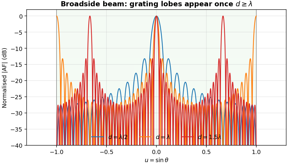
- At $d = lambda/2$ there is one beam, and the sidelobes stay low.
- At $d = lambda$ the grating lobes land exactly on $u = pm 1$, which is endfire (90°). They sit on the edge of visible space.
- At $d = 1.5lambda$ they move to $u = pm 2/3$, which is $pm 41.8^circ$. Those are full-height lobes you can see clearly.
Scanning makes it worse
Now steer the beam to $30^circ$, so $u_0 = 0.5$. Figure 2 compares two spacings.
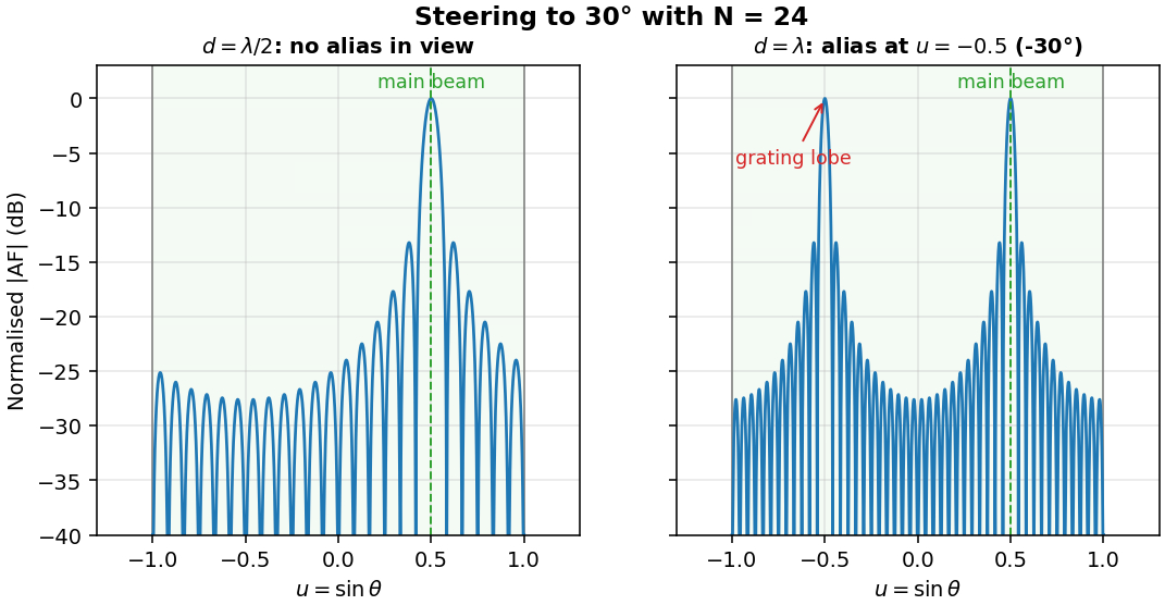
With $d = lambda/2$, the aliases sit at $u = 0.5 – 2 = -1.5$. Out of view, so the array is clean. With $d = lambda$, the alias sits at $u = 0.5 – 1 = -0.5$, which is $-30^circ$. Now the array radiates a second beam, mirror-image to the first.
Here is a worked case that surprised me the first time. Steer to $60^circ$:
- With $d = lambda$: $u_0 = sin 60^circ = 0.866$, so the alias is at $0.866 – 1 = -0.134$, which is $-7.7^circ$. The grating lobe sits only $7.7^circ$ from broadside.
- With $d = 0.6lambda$: the alias is at $0.866 – 1.667 = -0.801$, which is $-53.2^circ$.
- With $d = lambda/2$: the alias is at $0.866 – 2 = -1.134$. Out of view, so no problem.
For any scan angle $theta_0$, the largest spacing that keeps grating lobes out of view is
$$d_{max} = frac{lambda}{1 + |sintheta_0|}.$$
At $60^circ$ that gives $d_{max} = 0.536lambda$. So “a little over half a wavelength” is already too wide for a 60° scan.
The budget picture
Figure 3 plots the largest safe scan against spacing. The shaded area is the region you can use.
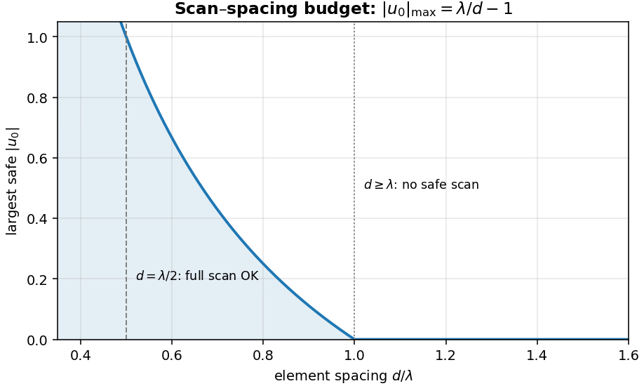
The curve reaches $|u_0| = 1$ at $d = lambda/2$ and falls to zero at $d = lambda$. Every design that goes wider than half a wavelength gives up part of its scan range.
How to avoid them in practice
- Set spacing from the highest frequency. Wavelength shrinks as frequency rises, so a band that runs to 30 GHz needs the spacing set at 30 GHz, not at the centre frequency. At 28 GHz, $lambda = 10.71$ mm, so $lambda/2 = 5.35$ mm. A 28 GHz array pitch of that size leaves no margin for error.
- Limit the scan range to what the spacing allows. A sector array with a 40° scan at $d = 0.6lambda$ is fine. The same array asked to scan 60° is not.
- Watch subarrays. Grouping elements into subarrays makes the effective spacing large. The grating lobes come back at the subarray pitch. Check them with pattern multiplication, which is the subject of the next article.
- Use the element pattern. Real elements are directional, and their pattern falls off near endfire. A grating lobe at $42^circ$ may be a few dB lower than the main beam after the element pattern is applied. That helps, but don’t count on it for lobes near endfire.
Python check
The snippet below prints the grating-lobe angles for any spacing and steering angle, and the largest safe scan for a range of spacings.
import numpy as np

def alias_angles(d_lam, theta0_deg):
    """Visible grating-lobe angles (degrees) for a uniform linear array."""
    u0 = np.sin(np.radians(theta0_deg))
    angles = []
    for m in range(-3, 4):
        if m == 0:
            continue                    # skip the main beam
        u = u0 + m / d_lam              # grating-lobe positions in u = sin(theta)
        if -1 <= u <= 1:
            angles.append(round(float(np.degrees(np.arcsin(u))), 1))
    return sorted(angles)

def max_safe_scan(d_lam):
    """Largest |theta0| (degrees) with no grating lobe in visible space."""
    x = 1 / d_lam - 1
    return 90.0 if x >= 1 else (round(float(np.degrees(np.arcsin(x))), 1) if x > 0 else 0.0)

print('d/lambda  max safe |u0|  max safe theta0 (deg)')
for d in (0.5, 0.6, 0.7, 0.8, 1.0):
    print(f'{d:8.1f}  {max(0, 1/d-1):14.3f}  {max_safe_scan(d):18.1f}')
print('d = lambda,   theta0 = 60 deg ->', alias_angles(1.0, 60))
print('d = 0.6 lambda, theta0 = 60 deg ->', alias_angles(0.6, 60))
print('d = lambda/2, theta0 = 60 deg ->', alias_angles(0.5, 60))
Output:
d/lambda  max safe |u0|  max safe theta0 (deg)
     0.5           1.000                90.0
     0.6           0.667                41.8
     0.7           0.429                25.4
     0.8           0.250                14.5
     1.0           0.000                 0.0
d = lambda,   theta0 = 60 deg -> [-7.7]
d = 0.6 lambda, theta0 = 60 deg -> [-53.2]
d = lambda/2, theta0 = 60 deg -> []
Questions readers often ask
Do grating lobes always ruin a design? Not always. If the element pattern is narrow enough to suppress the lobe, or the lobe falls outside the region you care about, it may be acceptable. But you have to check it. Don’t assume.
Does a grating lobe take power from the main beam? Yes. The array’s radiated power is shared among all its beams, so the main beam’s peak gain falls. The total radiated power is unchanged.
Keep learning
- Phased array antenna: an introduction: what a phased array is and why it steers.
- Electronic scanning arrays: the phase ramp that steers the beam.
- Array pattern multiplication: element pattern times array factor, with scan loss and tapering.
- Antenna factor and gain converter and FSPL and link budget calculator.
Want the complete Matlab labs? Path loss, fading and link-budget simulations are worked end to end in Wireless Communication Systems in Matlab. See all ebooks.
References
- C. A. Balanis, Antenna Theory: Analysis and Design, 4th ed., Wiley, 2016, Chapter 6 (arrays).
- R. J. Mailloux, Phased Array Antenna Handbook, 3rd ed., Artech House, 2017.
- S. J. Orfanidis, Electromagnetic Waves and Antennas, Rutgers University, free online edition, chapters on antenna arrays. eceweb1.rutgers.edu/~orfanidi/ewa