Auto-correlation, also called series correlation, is the correlation of a given sequence with itself as a function of time lag. Cross-correlation is a more generic term, which gives the correlation between two different sequences as a function of time lag.
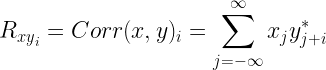
Given two sequences and , the cross-correlation at times separated by lag i is given by ( denotes complex conjugate operation)
Auto-correlation is a special case of cross-correlation, where x=y. One can use a brute force method (using for loops implementing the above equation) to compute the auto-correlation sequence. However, other alternatives are also at your disposal.
Method 1: Auto-correlation using xcorr function
Matlab
For a N-dimensional given vector x, the Matlab command xcorr(x,x) or simply xcorr(x) gives the auto-correlation sequence. For the input sequence x=[1,2,3,4], the command xcorr(x) gives the following result.
In Python, autocorrelation of 1-D sequence can be obtained using numpy.correlate function. Set the parameter mode=’full’ which is useful for calculating the autocorrelation as a function of lag.
import numpy as np
x = np.asarray([1,2,3,4])
np.correlate(x, x,mode='full')
# output: array([ 4, 11, 20, 30, 20, 11,  4])
Method 2: Auto-correlation using Convolution
Auto-correlation sequence can be computed as the convolution between the given sequence and the reversed (flipped) version of the conjugate of the sequence.The conjugate operation is not needed if the input sequence is real.
import numpy as np
x = np.asarray([1,2,3,4])
np.convolve(x,np.conj(x)[::-1])
# output: array([ 4, 11, 20, 30, 20, 11,  4])
Method 3: Autocorrelation using Toeplitz matrix
Autocorrelation sequence can be found using Toeplitz matrices. An example for using Toeplitz matrix structure for computing convolution is given here. The same technique is extended here, where one signal is set as input sequence and the other is just the flipped version of its conjugate. The conjugate operation is not needed if the input sequence is real.
import numpy as np
from scipy.linalg import toeplitz
x = np.asarray([1,2,3,4])
toeplitz(np.pad(x, (0,len(x)-1),mode='constant'),np.pad([x[0]], (0,len(x)-1),mode='constant'))@x[::-1]
# output: array([ 4, 11, 20, 30, 20, 11, 4])
Method 4: Auto-correlation using FFT/IFFT
Auto-correlation sequence can be found using FFT/IFFT pairs. An example for using FFT/IFFT for computing convolution is given here. The same technique is extended here, where one signal is set as input sequence and the other is just the flipped version of its conjugate.The conjugate operation is not needed if the input sequence is real.
import numpy as np
from scipy.fftpack import fft,ifft

x = np.asarray([1,2,3,4])

L = 2*len(x) - 1
ifft(fft(x,L)*fft(np.conj(x)[::-1],L))
#output: array([ 4+0j, 11+0j, 20+0j, 30+0j, 20+0j, 11+0j, 4+0j])
Note that in all the above cases, due to the symmetry property of auto-correlation function, the center element represents .
Construction the Auto-correlation Matrix
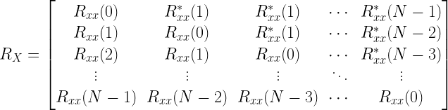
Auto-correlation matrix is a special form of matrix constructed from auto-correlation sequence. It takes the following form.
The auto-correlation matrix is easily constructed, once the auto-correlation sequence is known. The auto-correlation matrix is a Hermitian matrix as well as a Toeplitz matrix. This property is exploited in the following code for constructing the Auto-Correlation matrix.
Matlab
>> x=[1+j 2+j 3-j] %x is complex
>> acf=conv(x,fliplr(conj(x)))% %using Method 2 to compute Auto-correlation sequence
>>Rxx=acf(3:end); % R_xx(0) is the center element
>>Rx=toeplitz(Rxx,[Rxx(1) conj(Rxx(2:end))])
Python
import numpy as np
x = np.asarray([1+1j,2+1j,3-1j]) #x is complex
acf = np.convolve(x,np.conj(x)[::-1]) # using Method 2 to compute Auto-correlation sequence
Rxx=acf[2:]; # R_xx(0) is the center element
Rx = toeplitz(Rxx,np.hstack((Rxx[0], np.conj(Rxx[1:]))))
Result:
Rate this article: Note: There is a rating embedded within this post, please visit this post to rate it.
A random process (or signal for your visualization) with a constant power spectral density (PSD) function is a white noise process.
Power Spectral Density
Power Spectral Density function (PSD) shows how much power is contained in each of the spectral component. For example, for a sine wave of fixed frequency, the PSD plot will contain only one spectral component present at the given frequency. PSD is an even function and so the frequency components will be mirrored across the Y-axis when plotted. Thus for a sine wave of fixed frequency, the double sided plot of PSD will have two components – one at +ve frequency and another at –ve frequency of the sine wave. (Know how to plot PSD/FFT in Python & in Matlab)
Gaussian and Uniform White Noise:
A white noise signal (process) is constituted by a set of independent and identically distributed (i.i.d) random variables. In discrete sense, the white noise signal constitutes a series of samples that are independent and generated from the same probability distribution. For example, you can generate a white noise signal using a random number generator in which all the samples follow a given Gaussian distribution. This is called White Gaussian Noise (WGN) or Gaussian White Noise. Similarly, a white noise signal generated from a Uniform distribution is called Uniform White Noise.
Gaussian Noise and Uniform Noise are frequently used in system modelling. In modelling/simulation, white noise can be generated using an appropriate random generator. White Gaussian Noise can be generated using randn function in Matlab which generates random numbers that follow a Gaussian distribution. Similarly, rand function can be used to generate Uniform White Noise in Matlab that follows a uniform distribution. When the random number generators are used, it generates a series of random numbers from the given distribution. Let’s take the example of generating a White Gaussian Noise of length 10 using randn function in Matlab – with zero mean and standard deviation=1.
This simply generates 10 random numbers from the standard normal distribution. As we know that a white process is seen as a random process composing several random variables following the same Probability Distribution Function (PDF). The 10 random numbers above are generated from the same PDF (standard normal distribution). This condition is called “identically distributed” condition. The individual samples given above are “independent” of each other. Furthermore, each sample can be viewed as a realization of one random variable. In effect, we have generated a random process that is composed of realizations of 10 random variables. Thus, the process above is constituted from “independent identically distributed” (i.i.d) random variables.
Strictly and weakly defined white noise:
Since the white noise process is constructed from i.i.d random variable/samples, all the samples follow the same underlying probability distribution function (PDF). Thus, the Joint Probability Distribution function of the process will not change with any shift in time. This is called a stationary process. Hence, this noise is a stationary process. As with a stationary process which can be classified as Strict Sense Stationary (SSS) and Wide Sense Stationary (WSS) processes, we can have white noise that is SSS and white noise that is WSS. Correspondingly they can be called strictly defined white noise signal and weakly defined white noise signal.
What’s with Covariance Function/Matrix ?
A white noise signal, denoted by \(x(t)\), is defined in weak sense is a more practical condition. Here, the samples are statistically uncorrelated and identically distributed with some variance equal to \(\sigma^2\). This condition is specified by using a covariance function as
\[COV \left(x_i, x_j \right) = \begin{cases} \sigma^2, & \quad i = j \\ 0, & \quad i \neq j \end{cases}\]
Why do we need a covariance function? Because, we are dealing with a random process that is composed of \(n\) random variables (10 variables in the modelling example above). Such a process is viewed as multivariate random vector or multivariate random variable.
For multivariate random variables, Covariance function specified how each of the \(n\) variables in the given random process behaves with respect to each other. Covariance function generalizes the notion of variance to multiple dimensions.
The above equation when represented in the matrix form gives the covariance matrix of the white noise random process. Since the random variables in this process are statistically uncorrelated, the covariance function contains values only along the diagonal.
The matrix above indicates that only the auto-correlation function exists for each random variable. The cross-correlation values are zero (samples/variables are statistically uncorrelated with respect to each other). The diagonal elements are equal to the variance and all other elements in the matrix are zero.The ensemble auto-correlation function of the weakly defined white noise is given by This indicates that the auto-correlation function of weakly defined white noise process is zero everywhere except at lag \(\tau=0\).
\[R_{xx}(\tau) = E \left[ x(t) x^*(t-\tau)\right] = \sigma^2 \delta (\tau)\]
Wiener-Khintchine Theorem states that for Wide Sense Stationary Process (WSS), the power spectral density function \(S_{xx}(f)\) of a random process can be obtained by Fourier Transform of auto-correlation function of the random process. In continuous time domain, this is represented as
\[S_{xx}(f) = F \left[R_{xx}(\tau) \right] = \int_{-\infty}^{\infty} R_{xx} (\tau) e ^{- j 2 \pi f \tau} d \tau\]
For the weakly defined white noise process, we find that the mean is a constant and its covariance does not vary with respect to time. This is a sufficient condition for a WSS process. Thus we can apply Weiner-Khintchine Theorem. Therefore, the power spectral density of the weakly defined white noise process is constant (flat) across the entire frequency spectrum (Figure 1). The value of the constant is equal to the variance or power of the noise signal.
\[S_{xx}(f) = F \left[R_{xx}(\tau) \right] = \int_{-\infty}^{\infty} \sigma^2 \delta (\tau) e ^{- j 2 \pi f \tau} d \tau = \sigma^2 \int_{-\infty}^{\infty} \delta (\tau) e ^{- j 2 \pi f \tau} = \sigma^2\]
Figure 1: Weiner-Khintchine theorem illustrated
Testing the characteristics of White Gaussian Noise in Matlab:
Generate a Gaussian white noise signal of length \(L=100,000\) using the randn function in Matlab and plot it. Let’s assume that the pdf is a Gaussian pdf with mean \(\mu=0\) and standard deviation \(\sigma=2\). Thus the variance of the Gaussian pdf is \(\sigma^2=4\). The theoretical PDF of Gaussian random variable is given by
subplot(2,1,2)
n=100; %number of Histrogram bins
[f,x]=hist(X,n);
bar(x,f/trapz(x,f)); hold on;
%Theoretical PDF of Gaussian Random Variable
g=(1/(sqrt(2*pi)*sigma))*exp(-((x-mu).^2)/(2*sigma^2));
plot(x,g);hold off; grid on;
title('Theoretical PDF and Simulated Histogram of White Gaussian Noise');
legend('Histogram','Theoretical PDF');
xlabel('Bins');
ylabel('PDF f_x(x)');
Figure 3: Plot of simulated & theoretical PDF for Gaussian RV
Compute the auto-correlation function of the white noise. The computed auto-correlation function has to be scaled properly. If the ‘xcorr’ function (inbuilt in Matlab) is used for computing the auto-correlation function, use the ‘biased’ argument in the function to scale it properly.
figure();
Rxx=1/L*conv(flipud(X),X);
lags=(-L+1):1:(L-1);

%Alternative method
%[Rxx,lags] =xcorr(X,'biased');
%The argument 'biased' is used for proper scaling by 1/L
%Normalize auto-correlation with sample length for proper scaling

plot(lags,Rxx);
title('Auto-correlation Function of white noise');
xlabel('Lags')
ylabel('Correlation')
grid on;
Figure 4: Autocorrelation function of generated noise
Simulating the PSD:
Simulating the Power Spectral Density (PSD) of the white noise is a little tricky business. There are two issues here 1) The generated samples are of finite length. This is synonymous to applying truncating an infinite series of random samples. This implies that the lags are defined over a fixed range. ( FFT and spectral leakage – an additional resource on this topic can be found here) 2) The random number generators used in simulations are pseudo-random generators. Due these two reasons, you will not get a flat spectrum of psd when you apply Fourier Transform over the generated auto-correlation values.The wavering effect of the psd can be minimized by generating sufficiently long random signal and averaging the psd over several realizations of the random signal.
Simulating Gaussian White Noise as a Multivariate Gaussian Random Vector:
To verify the power spectral density of the white noise, we will use the approach of envisaging the noise as a composite of \(N\) Gaussian random variables. We want to average the PSD over \(L\) such realizations. Since there are \(N\) Gaussian random variables (\(N\) individual samples) per realization, the covariance matrix \( C_{xx}\) will be of dimension \(N \times N\). The vector of mean for this multivariate case will be of dimension \(1 \times N\).
Cholesky decomposition of covariance matrix gives the equivalent standard deviation for the multivariate case. Cholesky decomposition can be viewed as square root operation. Matlab’s randn function is used here to generate the multi-dimensional Gaussian random process with the given mean matrix and covariance matrix.
%Verifying the constant PSD of White Gaussian Noise Process
%with arbitrary mean and standard deviation sigma

mu=0; %Mean of each realization of Noise Process
sigma=2; %Sigma of each realization of Noise Process

L = 1000; %Number of Random Signal realizations to average
N = 1024; %Sample length for each realization set as power of 2 for FFT

%Generating the Random Process - White Gaussian Noise process
MU=mu*ones(1,N); %Vector of mean for all realizations
Cxx=(sigma^2)*diag(ones(N,1)); %Covariance Matrix for the Random Process
R = chol(Cxx); %Cholesky of Covariance Matrix
%Generating a Multivariate Gaussian Distribution with given mean vector and
%Covariance Matrix Cxx
z = repmat(MU,L,1) + randn(L,N)*R;
Compute PSD of the above generated multi-dimensional process and average it to get a smooth plot.
%By default, FFT is done across each column - Normal command fft(z)
%Finding the FFT of the Multivariate Distribution across each row
%Command - fft(z,[],2)
Z = 1/sqrt(N)*fft(z,[],2); %Scaling by sqrt(N);
Pzavg = mean(Z.*conj(Z));%Computing the mean power from fft

normFreq=[-N/2:N/2-1]/N;
Pzavg=fftshift(Pzavg); %Shift zero-frequency component to center of spectrum
plot(normFreq,10*log10(Pzavg),'r');
axis([-0.5 0.5 0 10]); grid on;
ylabel('Power Spectral Density (dB/Hz)');
xlabel('Normalized Frequency');
title('Power spectral density of white noise');
Figure 5: Power spectral density of generated noise
The PSD plot of the generated noise shows almost fixed power in all the frequencies. In other words, for a white noise signal, the PSD is constant (flat) across all the frequencies (\(- \infty\) to \(+\infty\)). The y-axis in the above plot is expressed in dB/Hz unit. We can see from the plot that the \(constant \; power = 10 log_{10}(\sigma^2) = 10 log_{10}(4) = 6\; dB\).
Application
In channel modeling, we often come across additive white Gaussian noise (AWGN) channel. To know more about the channel model and its simulation, continue reading this article: Simulate AWGN channel in Matlab & Python.
Rate this article: Note: There is a rating embedded within this post, please visit this post to rate it.
Note: There is a rating embedded within this post, please visit this post to rate it.
The following is a function to generate a Walsh Hadamard Matrix of given codeword size. The codeword size has to be a power of 2.
function [H]=generateHadamardMatrix(codeSize)

%[H]=generateHadamardMatrix(codeSize);
% Function to generate Walsh-Hadamard Matrix where "codeSize" is the code
% length of walsh code. The first matrix gives us two codes; 00, 01. The second
% matrix gives: 0000, 0101, 0011, 0110 and so on
% Author: Mathuranathan for https://www.gaussianwaves.com
% License: Creative Commons: Attribution-NonCommercial-ShareAlike 3.0
% Unported

%codeSize=64; %For testing only
N=2;
H=[0 0 ; 0 1];
if bitand(codeSize,codeSize-1)==0
while(N~=codeSize)
       N=N*2;
       H=repmat(H,[2,2]);
       [m,n]=size(H);

      %Invert the matrix located at the bottom right hand corner
      for i=m/2+1:m,
          for j=n/2+1:n,
                H(i,j)=~H(i,j);
         end
     end
end
else
disp('INVALID CODE SIZE:The code size must be a power of 2');
end
Example:
To Generate Walsh Codes used in IS-95 (which utilizes 64 Walsh codes of size 64 bits each, use : [H]=generateHadamardMatrix(64). This will generate 64 Walsh Codes of length 64-bits (for each code).
Test Program:
Click Here to download
Also given below is a program to test the cross-correlation and auto-correlation of Walsh code. A set of 8-Walsh codes are used for this purpose.
% Matlab Program to test Walsh Hadamard Codes and to test their orthogonality
% Plots cross-correlation and auto correlation of Walsh Hadamard Codes
% Author: Mathuranathan Viswanathan for https://www.gaussianwaves.com
% License: Creative Commons: Attribution-NonCommercial-ShareAlike 3.0
% Unported

codeSize=8;
[H]=generateHadamardMatrix(codeSize);

%-----------------------------------------------------------
%Cross-Correlation of Walsh Code 1 with rest of Walsh Codes
h = zeros(1, codeSize-1); %For dynamic Legends
s = cell(1, codeSize-1); %For dynamic Legends
for rows=2:codeSize
[crossCorrelation,lags]=crossCorr(H(1,:),H(rows,:));
h(rows-1)=plot(lags,crossCorrelation);
s{rows-1} = sprintf('Walsh Code Sequence #-%d', rows);
hold all;
end

%Dynamic Legends
% Select the plots to include in the legend
index = 1:codeSize-1;

% Create legend for the selected plots
legend(h(index),s{index});
title('Cross Correlation of Walsh Code 1 with the rest of the Walsh Codes');
ylabel('Cross Correlation');
xlabel('Lags');

%-----------------------------------------------------------
%AutoCorrelation of Walsh Code - 1
autoCorr2(H(2,:),8,2,1);
Simulation Results
From the plots below, it can be ascertained that the Walsh codes has excellent cross-correlation property and poor autocorrelation property. Excellent cross-correlation property (zero cross-correlation) implies orthogonality, which makes it suitable for CDMA applications.
This website uses cookies to improve your experience while you navigate through the website. Out of these, the cookies that are categorized as necessary are stored on your browser as they are essential for the working of basic functionalities of the website. We also use third-party cookies that help us analyze and understand how you use this website. These cookies will be stored in your browser only with your consent. You also have the option to opt-out of these cookies. But opting out of some of these cookies may affect your browsing experience.
Necessary cookies are absolutely essential for the website to function properly. These cookies ensure basic functionalities and security features of the website, anonymously.
Cookie
Duration
Description
cookielawinfo-checbox-analytics
11 months
This cookie is set by GDPR Cookie Consent plugin. The cookie is used to store the user consent for the cookies in the category "Analytics".
cookielawinfo-checbox-analytics
11 months
This cookie is set by GDPR Cookie Consent plugin. The cookie is used to store the user consent for the cookies in the category "Analytics".
cookielawinfo-checbox-functional
11 months
The cookie is set by GDPR cookie consent to record the user consent for the cookies in the category "Functional".
cookielawinfo-checbox-functional
11 months
The cookie is set by GDPR cookie consent to record the user consent for the cookies in the category "Functional".
cookielawinfo-checbox-others
11 months
This cookie is set by GDPR Cookie Consent plugin. The cookie is used to store the user consent for the cookies in the category "Other.
cookielawinfo-checbox-others
11 months
This cookie is set by GDPR Cookie Consent plugin. The cookie is used to store the user consent for the cookies in the category "Other.
cookielawinfo-checkbox-necessary
11 months
This cookie is set by GDPR Cookie Consent plugin. The cookies is used to store the user consent for the cookies in the category "Necessary".
cookielawinfo-checkbox-performance
11 months
This cookie is set by GDPR Cookie Consent plugin. The cookie is used to store the user consent for the cookies in the category "Performance".
viewed_cookie_policy
11 months
The cookie is set by the GDPR Cookie Consent plugin and is used to store whether or not user has consented to the use of cookies. It does not store any personal data.
Functional cookies help to perform certain functionalities like sharing the content of the website on social media platforms, collect feedbacks, and other third-party features.
Performance cookies are used to understand and analyze the key performance indexes of the website which helps in delivering a better user experience for the visitors.
Analytical cookies are used to understand how visitors interact with the website. These cookies help provide information on metrics the number of visitors, bounce rate, traffic source, etc.