Understand various characteristics of a wireless channel through multipath channel models. Discuss Wide Sense Stationary channel, uncorrelated scattering channel, wide sense stationary uncorrelated scattering channel models and scattering function.
Introduction
Wireless channel is of time-varying nature in which the parameters randomly change with respect to time. Wireless channel is very harsh when compared to AWGN channel model which is often considered for simulation and modeling. Understanding the various characteristics of a wireless channel and understanding their physical significance is of paramount importance. In these series of articles, I seek to expound various statistical characteristics of a multipath wireless channel by giving more importance to the concept than the mathematical derivation.
[table “36” not found /]
Complex baseband mutipath channel model:
In a multipath channel, multiple copies of a signal travel different paths with different propagation delays $latex \tau$ and are received at the receiver at different phase angles and strengths. These rays add constructively or destructively at the receiver front end, thereby giving rise to rapid fluctuations in the channel. The multipath channel can be viewed as a linear time variant system where the parameters change randomly with respect to time. The channel impulse response is a two dimensional random variable – $latex h(t, \tau)$ that is a function of two parameters – instantaneous time $latex t$ and the propagation delay $latex \tau$. The channel is expressed as a set of random complex gains at a given time $latex t$ and the propagation delay $latex \tau$. The output of the channel $latex y(t)$ can be expressed as the convolution of the complex channel impulse response $latex h(t, \tau)$ and the input $latex x(t)$
$latex y(t) = \int_{0}^{\infty } h(t – \tau, \tau) x(t- \tau) d \tau \quad\quad (1) &s=2$
If the complex channel gains are typically drawn from a complex Gaussian distribution, then at any given time $latex t$, the absolute value of the impulse response $latex \left| h(t,\tau) \right| $ is Rayleigh distributed (if the mean of the distribution $latex E\left ( h(t,\tau) \right)=0$ or Rician distributed (if the mean of the distribution $latex E\left [ h(t,\tau) \right ) \neq 0] $. These two scenarios model the presence or absence of a Line of Sight (LOS) path between the transmitter and the receiver.
Here, the values for the channel impulse response are samples of a random process that is defined with respect to time $latex t$ and the multipath delay τ. That is, for each combination of $latex t$ and τ, a randomly drawn value is assigned for the channel impulse response. As with any other random process, we can calculate the general autocorrelation function as
$latex R_{hh}(t_1,t_2;\tau_1,\tau_2)= E\left [ h(t_1,\tau_1)h^*(t_2,\tau_2) \right ] \quad\quad (2) &s=2$
Given the generic autocorrelation function above, following assumptions can be made to restrict the channel model to the following specific set of categories
- Wide Sense Stationary channel model
- Uncorrelated Scattering channel model
- Wide Sense Stationary Uncorrelated Scattering channel model
Wide Sense Stationary (WSS) channel model
In this channel model, the impulse response of the channel is considered Wide Sense Stationary (WSS) , that is the channel impulse response is independent of time $latex t$. In other words, the autocorrelation function $latex R_{hh}(t,\tau)$ is independent of time instant \(t\) and it depends on the difference between the time instants $latex \Delta t=t_2-t_1$ where $latex t_1=t$ and $latex t_2=t+\Delta t$. The autocorrelation function for WSS channel model is expressed as
$latex R_{hh} (\Delta t ; \tau_1,\tau_2)= E\left[ h(t,\tau_1) h^\ast (t+\Delta t,\tau_2) \right] \quad\quad (3) &s=2$
Uncorrelated Scattering (US) channel model
Here, the individual scattered components arriving at the receiver front end (at different propagation delays) are assumed to be uncorrelated. Thus the autocorrelation function can be expressed as
$latex R_{hh}(t_1, t_2 ; \tau_1,\tau_2 )= R_{hh} ( t_1, t_2 ; \tau_1 ) \delta ( \tau_1- \tau_2) \quad\quad (4) &s=2$
Wide Sense Stationary Uncorrelated Scattering (WSSUS) channel model
The WSSUS channel model combines the aspects of WSS and US channel model that are discussed above. Here, the channel is considered as Wide Sense Stationary and the scattering components arriving at the receiver are assumed to be uncorrelated. Combining both the worlds, the autocorrelation function $latex R_{hh}(\Delta t,\tau)$is
$latex R_{hh}(\Delta t ,\tau )=E\left[ h(t,\tau)h^\ast (t+\Delta t,\tau) \right] \quad\quad (5) &s=2$
Scattering function
The autocorrelation function of the WSSUS channel model can be represented in frequency domain by taking Fourier transform with respect one or both variables – difference in time $latex \Delta t$ and the propagation delay $latex \tau$. Of the two forms, the Fourier transform on the variable $latex \Delta t$ gives specific insight to channel properties in terms of propagation delay $latex \tau$ and the Doppler Frequency $latex f$ simultaneously. The Fourier transform of the above two-dimensional autocorrelation function on the variable $latex \Delta t$ is called scattering function and is given by
$latex S(f,\tau)=\int_{-\infty }^{\infty }R_{hh}(\Delta t, \tau)e^{-j2 \pi f \Delta t} d \Delta t \quad\quad (6) &s=2$
Fourier transform of relative time $latex \Delta t$ is Doppler Frequency. Thus, the scattering function is a function of two variables – Dopper Frequency $latex f$ and the propagation delay $latex \tau$. It gives the average output power of the channel as a function of Doppler Frequency $latex f$ and the propagation delay $latex \tau$.
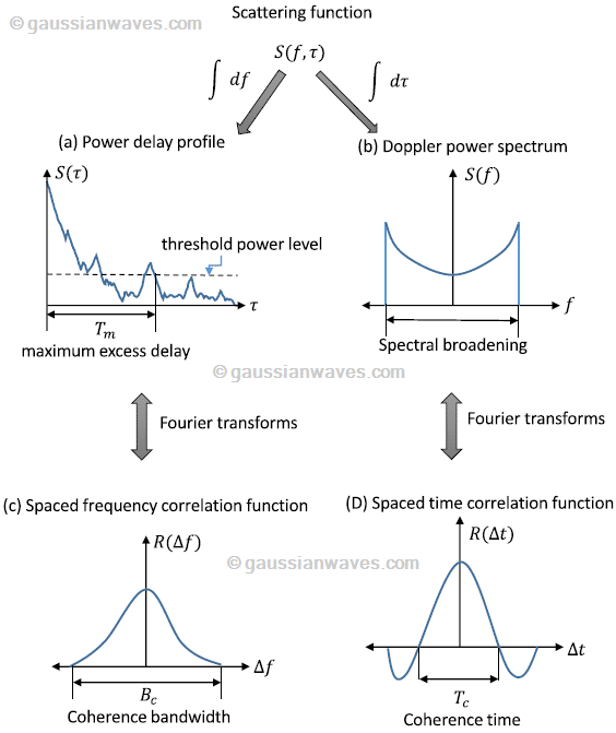
Two important relationships can be derived from the scattering function – Power Delay Profile (PDP) and Doppler Power Spectrum. Both of them affect the performance of a given wireless channel. Power Delay Profile is a function of propagation delay and the Doppler Power Spectrum is a function of Doppler Frequency.
Power Delay Profile $latex p(\tau)$ gives the signal intensity received over a multipath channel as a function of propagation delays. It is obtained as the spatial average of the complex baseband channel impulse response as
$latex p(\tau) = R_{hh}(0,\tau)= E\left [ \left | h(t,\tau) \right | ^2 \right ] \quad\quad (7) &s=2$
Power Delay Profile can also be obtained from scattering function, by integrating it over the entire frequency range (removing the dependence on Doppler frequency).
$latex p(\tau) = \int_{-\infty }^{\infty } S(f,\tau) df \quad\quad (8) &s=2$
Similarly, the Doppler Power Spectrum can be obtained by integrating the scattering function over the entire range of propagation delays.
$latex S(f) = \int_{-\infty }^{\infty } S(f,\tau) d \tau \quad\quad (9) &s=2$
Fourier Transform of Power Delay Profile and Inverse Fourier Transform of Doppler Power Spectrum:
Power Delay Profile is a function of time which can be transformed to frequency domain by taking Fourier Transform. Fourier Transform of Power Delay Profile is called spaced-frequency correlation function. Spaced-frequency correlation function describes the spreading of a signal in frequency domain. This gives rise to the importance channel parameter – Coherence Bandwidth.
Similarly, the Doppler Power Spectrum describes the output power of the multipath channel in frequency domain. The Doppler Power Spectrum when translated to time-domain by means of inverse Fourier transform is called spaced-time correlation function. Spaced-time correlation function describes the correlation between different scattered signals received at two different times as a function of the difference in the received time. It gives rise to the concept of Coherence Time.
Next Topic : Power Delay Profile
Rate this article: [ratings]
For further reading
Books by the author
[table “23” not found /]
sir i am using energy detection based cooperative environment and have been calculating decision of each user in matlab simulink. Though i implemented the same using AWGN channel but when i use rayeligh fading block in the model, the problem occurs:
Complex signal mismatch. Input port 1 of ‘cooperative_110/SU_2/Multipath Rayleigh Fading Channel/Channel Filter’ expects a signal of numeric type complex. However, it is driven by a signal of numeric type real
Component: Simulink | Category: Block errorOpen
Complex signal mismatch. Output port 1 of ‘cooperative_110/SU_2/Multipath Rayleigh Fading Channel/In’ is a signal of numeric type real. However, it is driving a signal of numeric type complex
Though i tried to eradicate them using imag to real block but found no success..
Please help!!
Please try Matlab Central forum for resolving for software configuration errors. The same issue is discussed here.
https://www.mathworks.com/matlabcentral/newsreader/view_thread/132128
What happens to the delta function, isn’t is supposed to blow up at tou1=tou2 ?
I think, the dirac delta function is referred here (in the equation 4 above).
when τ1 = τ2 ==> δ(τ1 – τ2) = δ(0) = 1
Hi, thanks for sharing the topic. One suggestion related to the Figure 1 is that actually, the Time Correlation Function is the Inverse Fourier transform of the Doppler Spectrum Function (transfer from frequency domain to time domain). Figure 1 is a very good summary, however if you know mind please add the “Inverse Fourier transform” hint to the figure. Thank you.
Thanks for the suggestions.