Plot FFT using Python – FFT of sine wave & cosine wave

Key focus: Learn how to plot FFT of sine wave and cosine wave using Python. Understand FFTshift. Plot one-sided, double-sided and normalized spectrum using FFT.

Introduction

Numerous texts are available to explain the basics of Discrete Fourier Transform and its very efficient implementation – Fast Fourier Transform (FFT).  Often we are confronted with the need to generate simple, standard signals (sine, cosine, Gaussian pulse, squarewave, isolated rectangular pulse, exponential decay, chirp signal) for simulation purpose. I intend to show (in a series of articles) how these basic signals can be generated in Python and how to represent them in frequency domain using FFT. If you are inclined towards Matlab programming, visit here.

This article is part of the book Digital Modulations using Python, ISBN: 978-1712321638 available in ebook (PDF) and Paperback (hardcopy) formats

Sine Wave

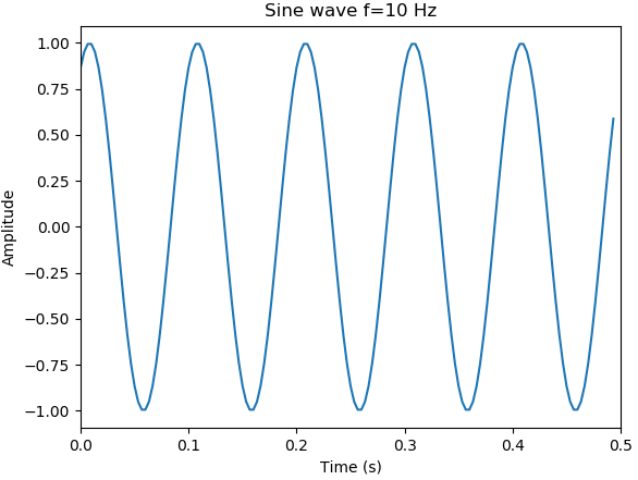
In order to generate a sine wave, the first step is to fix the frequency f of the sine wave. For example, we wish to generate a sine wave whose minimum and maximum amplitudes are -1V and +1V respectively. Given the frequency of the sinewave, the next step is to determine the sampling rate.

For baseband signals, the sampling is straight forward. By Nyquist Shannon sampling theorem, for faithful reproduction of a continuous signal in discrete domain, one has to sample the signal at a rate higher than at-least twice the maximum frequency contained in the signal (actually, it is twice the one-sided bandwidth occupied by a real signal. For a baseband signal bandwidth ( to ) and maximum frequency in a given band are equivalent).

For Python implementation, let us write a function to generate a sinusoidal signal using the Python’s Numpy library. Numpy is a fundamental library for scientific computations in Python. In order to use the numpy package, it needs to be imported. Here, we are importing the numpy package and renaming it as a shorter alias np.

import numpy as np

Next, we define a function for generating a sine wave signal with the required parameters.

def sine_wave(f,overSampRate,phase,nCyl):
	"""
	Generate sine wave signal with the following parameters
	Parameters:
		f : frequency of sine wave in Hertz
		overSampRate : oversampling rate (integer)
		phase : desired phase shift in radians
		nCyl : number of cycles of sine wave to generate
	Returns:
		(t,g) : time base (t) and the signal g(t) as tuple
	Example:
		f=10; overSampRate=30;
		phase = 1/3*np.pi;nCyl = 5;
		(t,g) = sine_wave(f,overSampRate,phase,nCyl)
	"""
	fs = overSampRate*f # sampling frequency
	t = np.arange(0,nCyl*1/f-1/fs,1/fs) # time base
	g = np.sin(2*np.pi*f*t+phase) # replace with cos if a cosine wave is desired
	return (t,g) # return time base and signal g(t) as tuple

We note that the function sine wave is defined inside a file named signalgen.py. We will add more such similar functions in the same file. The intent is to hold all the related signal generation functions, in a single file. This approach can be extended to object oriented programming. Now that we have defined the sine wave function in signalgen.py, all we need to do is call it with required parameters and plot the output.

"""
Simulate a sinusoidal signal with given sampling rate
"""
import numpy as np
import matplotlib.pyplot as plt # library for plotting
from signalgen import sine_wave # import the function

f = 10 #frequency = 10 Hz
overSampRate = 30 #oversammpling rate
fs = f*overSampRate #sampling frequency
phase = 1/3*np.pi #phase shift in radians
nCyl = 5 # desired number of cycles of the sine wave

(t,x) = sine_wave(f,overSampRate,phase,nCyl) #function call

plt.plot(t,x) # plot using pyplot library from matplotlib package
plt.title('Sine wave f='+str(f)+' Hz') # plot title
plt.xlabel('Time (s)') # x-axis label
plt.ylabel('Amplitude') # y-axis label
plt.show() # display the figure

Python is an interpreter based software language that processes everything in digital. In order to obtain a smooth sine wave, the sampling rate must be far higher than the prescribed minimum required sampling rate, that is at least twice the frequency – as per Nyquist-Shannon theorem. Hence, we need to sample the input signal at a rate significantly higher than what the Nyquist criterion dictates. Higher oversampling rate requires more memory for signal storage. It is advisable to keep the oversampling factor to an acceptable value.

An oversampling factor of is chosen in the previous function. This is to plot a smooth continuous like sine wave. Thus, the sampling rate becomes . If a phase shift is desired for the sine wave, specify it too.

Different representations of FFT:

Since FFT is just a numeric computation of -point DFT, there are many ways to plot the result. The FFT, implemented in Scipy.fftpack package, is an algorithm published in 1965 by J.W.Cooley and
J.W.Tuckey for efficiently calculating the DFT.

The SciPy functions that implement the FFT and IFFT can be invoked as follows

from scipy.fftpack import fft, ifft
X = fft(x,N) #compute X[k]
x = ifft(X,N) #compute x[n]

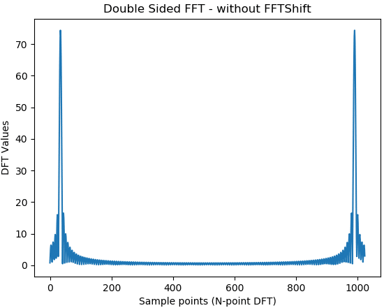
1. Plotting raw values of DFT:

The x-axis runs from to – representing sample values. Since the DFT values are complex, the magnitude of the DFT is plotted on the y-axis. From this plot we cannot identify the frequency of the sinusoid that was generated.

import numpy as np
import matplotlib.pyplot as plt
from scipy.fftpack import fft

NFFT=1024 #NFFT-point DFT      
X=fft(x,NFFT) #compute DFT using FFT    

fig1, ax = plt.subplots(nrows=1, ncols=1) #create figure handle
nVals = np.arange(start = 0,stop = NFFT) # raw index for FFT plot
ax.plot(nVals,np.abs(X))      
ax.set_title('Double Sided FFT - without FFTShift')
ax.set_xlabel('Sample points (N-point DFT)')        
ax.set_ylabel('DFT Values')
fig1.show()

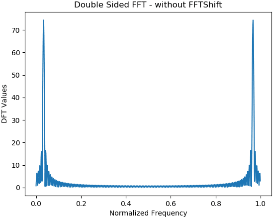
2. FFT plot – plotting raw values against normalized frequency axis:

In the next version of plot, the frequency axis (x-axis) is normalized to unity. Just divide the sample index on the x-axis by the length of the FFT. This normalizes the x-axis with respect to the sampling rate . Still, we cannot figure out the frequency of the sinusoid from the plot.

import numpy as np
import matplotlib.pyplot as plt
from scipy.fftpack import fft

NFFT=1024 #NFFT-point DFT  
X=fft(x,NFFT) #compute DFT using FFT     

fig2, ax = plt.subplots(nrows=1, ncols=1) #create figure handle
   
nVals=np.arange(start = 0,stop = NFFT)/NFFT #Normalized DFT Sample points         
ax.plot(nVals,np.abs(X))     
ax.set_title('Double Sided FFT - without FFTShift')        
ax.set_xlabel('Normalized Frequency')
ax.set_ylabel('DFT Values')
fig2.show()

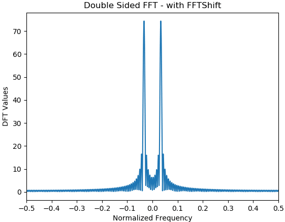
3. FFT plot – plotting raw values against normalized frequency (positive & negative frequencies):

As you know, in the frequency domain, the values take up both positive and negative frequency axis. In order to plot the DFT values on a frequency axis with both positive and negative values, the DFT value at sample index has to be centered at the middle of the array. This is done by using FFTshift function in Scipy Python. The x-axis runs from to where the end points are the normalized ‘folding frequencies’ with respect to the sampling rate .

import numpy as np
import matplotlib.pyplot as plt
from scipy.fftpack import fft,fftshift

NFFT=1024 #NFFT-point DFT      
X=fftshift(fft(x,NFFT)) #compute DFT using FFT  

fig3, ax = plt.subplots(nrows=1, ncols=1) #create figure handle
    
fVals=np.arange(start = -NFFT/2,stop = NFFT/2)/NFFT #DFT Sample points        
ax.plot(fVals,np.abs(X))
ax.set_title('Double Sided FFT - with FFTShift')
ax.set_xlabel('Normalized Frequency')
ax.set_ylabel('DFT Values');
ax.autoscale(enable=True, axis='x', tight=True)
ax.set_xticks(np.arange(-0.5, 0.5+0.1,0.1))
fig.show()

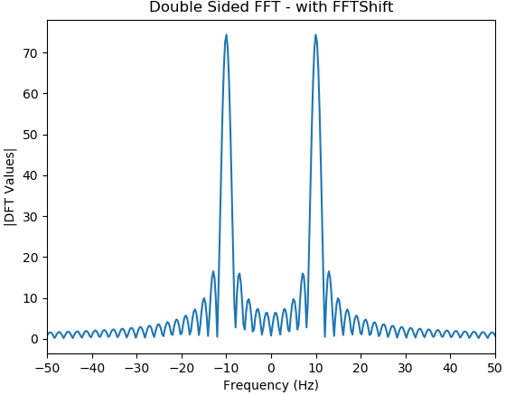
4. FFT plot – Absolute frequency on the x-axis vs. magnitude on y-axis:

Here, the normalized frequency axis is just multiplied by the sampling rate. From the plot below we can ascertain that the absolute value of FFT peaks at and . Thus the frequency of the generated sinusoid is . The small side-lobes next to the peak values at and are due to spectral leakage.

import numpy as np
import matplotlib.pyplot as plt
from scipy.fftpack import fft,fftshift

NFFT=1024     
X=fftshift(fft(x,NFFT))

fig4, ax = plt.subplots(nrows=1, ncols=1) #create figure handle

fVals=np.arange(start = -NFFT/2,stop = NFFT/2)*fs/NFFT
ax.plot(fVals,np.abs(X),'b')
ax.set_title('Double Sided FFT - with FFTShift')
ax.set_xlabel('Frequency (Hz)')         
ax.set_ylabel('|DFT Values|')
ax.set_xlim(-50,50)
ax.set_xticks(np.arange(-50, 50+10,10))
fig4.show()

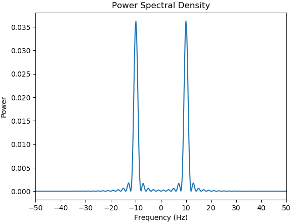
5. Power Spectrum – Absolute frequency on the x-axis vs. power on y-axis:

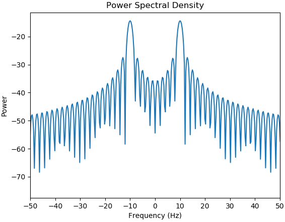
The following is the most important representation of FFT. It plots the power of each frequency component on the y-axis and the frequency on the x-axis. The power can be plotted in linear scale or in log scale. The power of each frequency component is calculated as

Where is the frequency domain representation of the signal . In Python, the power has to be calculated with proper scaling terms.

Plotting the PSD plot with y-axis on log scale, produces the most encountered type of PSD plot in signal processing.

Rate this article: (14 votes, average: 4.29 out of 5)

Books by the author

Wireless Communication Systems in Matlab Second Edition(PDF) Note: There is a rating embedded within this post, please visit this post to rate it. $14.99 – Add to Cart Checkout Added to cart	Digital Modulations using Python (PDF ebook) Note: There is a rating embedded within this post, please visit this post to rate it. $14.99 – Add to Cart Checkout Added to cart	Digital Modulations using Matlab (PDF ebook) Note: There is a rating embedded within this post, please visit this post to rate it. $14.99 – Add to Cart Checkout Added to cart
Hand-picked Best books on Communication Engineering Best books on Signal Processing

Topics in this chapter

Essentials of Signal Processing ● Generating standard test signals  □ Sinusoidal signals  □ Square wave  □ Rectangular pulse  □ Gaussian pulse  □ Chirp signal ● Interpreting FFT results - complex DFT, frequency bins and FFTShift  □ Real and complex DFT  □ Fast Fourier Transform (FFT)  □ Interpreting the FFT results  □ FFTShift  □ IFFTShift ● Obtaining magnitude and phase information from FFT  □ Discrete-time domain representation  □ Representing the signal in frequency domain using FFT  □ Reconstructing the time domain signal from the frequency domain samples ● Power spectral density ● Power and energy of a signal  □ Energy of a signal  □ Power of a signal  □ Classification of signals  □ Computation of power of a signal - simulation and verification ● Polynomials, convolution and Toeplitz matrices  □ Polynomial functions  □ Representing single variable polynomial functions  □ Multiplication of polynomials and linear convolution  □ Toeplitz matrix and convolution ● Methods to compute convolution  □ Method 1: Brute-force method  □ Method 2: Using Toeplitz matrix  □ Method 3: Using FFT to compute convolution  □ Miscellaneous methods ● Analytic signal and its applications  □ Analytic signal and Fourier transform  □ Extracting instantaneous amplitude, phase, frequency  □ Phase demodulation using Hilbert transform ● Choosing a filter : FIR or IIR : understanding the design perspective  □ Design specification  □ General considerations in design