In wireless environments, transmitted signal may be subjected to multiple scatterings before arriving at the receiver. This gives rise to random fluctuations in the received signal and this phenomenon is called fading. The scattered version of the signal is designated as non line of sight (NLOS) component. If the number of NLOS components are sufficiently large, the fading process is approximated as the sum of large number of complex Gaussian process whose probability-density-function follows Rayleigh distribution.
Rayleigh distribution is well suited for the absence of a dominant line of sight (LOS) path between the transmitter and the receiver. If a line of sight path do exist, the envelope distribution is no longer Rayleigh, but Rician (or Ricean). If there exists a dominant LOS component, the fading process can be represented as the sum of complex exponential and a narrowband complex Gaussian process g(t). If the LOS component arrive at the receiver at an angle of arrival(AoA)θ, phase ɸ and with the maximum Doppler frequency fD, the fading process in baseband can be represented as (refer [1])
where, K represents the Rician K factor given as the ratio of power of the LOS component A2 to the power of the scattered components (S2) marked in the equation above.
\[K=\frac{A^2}{S^2}\]
The received signal power Ω is the sum of power in LOS component and the power in scattered components, given as Ω=A2+S2. The above mentioned fading process is called Rician fading process. The best and worst-case Rician fading channels are associated with K=∞ and K=0 respectively. A Ricean fading channel with K=∞ is a Gaussian channel with a strong LOS path. Ricean channel with K=0 represents a Rayleigh channel with no LOS path.
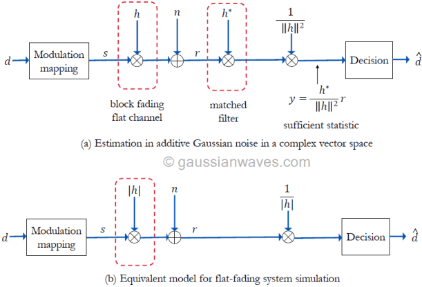
Figure 1: Simulation model for modulation and detection over flat fading channel
Simulation and performance results
In chapter 5 of the book Wireless communication systems in Matlab, the code implementation for complex baseband models for various digital modulators and demodulator are given. The computation and generation of AWGN noise is also given in the book. Using these models, we can create a unified simulation for code for simulating the performance of various modulation techniques over Rician flat-fading channel the simulation model shown in Figure 1(b).
An unified approach is employed to simulate the performance of any of the given modulation technique – MPSK, MQAM or MPAM. The simulation code (given in the book) will automatically choose the selected modulation type, performs Monte Carlo simulation, computes symbol error rates and plots them against the theoretical symbol error rate curves. The simulated performance results obtained for various modulations are shown in the Figure 2.
Figure 2: Performance of various modulations over Ricean flat fading channel
Rate this article: Note: There is a rating embedded within this post, please visit this post to rate it.
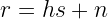
Assuming flat slow fading channel, the received signal model is given by
where, is the channel impulse response, is the received signal, is the transmitted signal and is the additive Gaussian white noise.
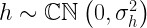
Assuming small scale Rayleigh fading, the channel impulse response is modeled as complex Gaussian random variable with zero mean and variance
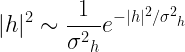
Therefore, the instantaneous channel power is exponentially distributed
In the context of AWGN channel, the signal-to-noise ratio (SNR) for a given channel condition, is a constant. But in the case of fading channels, the signal-to-noise ratio is no longer a constant as the signal is fluctuating when passed through a fading channel. Therefore, for fading channel, the SNR has a random variable component built into it. Hence, we just don’t call it SNR, instead it is called instantaneous SNR which depends on the current conditions of the channel (or equivalently, the value of the random variable at that instant). Since the SNR is a random variable, we can also talk about its expected (average) value, which is called average SNR. Denoting the average SNR as and for convenience, let’s assume that the average power of the channel is unity, i.e,
The instantaneous SNR is given by
Therefore, like the channel impulse response, the instantaneous SNR is also exponentially distributed
Maximum Ratio Combining (MRC)
The selection combining technique is the simplest technique, where in, the received signal from the antenna that experiences the highest SNR (i.e, the strongest signal from N received signals) is chosen for processing at the receiver. Therefore this technique throws away of observations. Whereas, in maximum ratio combining (MRC) all observations are used.
MRC works on the signal in spatial domain and is very similar to what a matched filter in frequency domain does to the incoming signal. MRC maximizes the inner product of the weights and the signal vector.
Figure 1: Processing the received samples at the receiver
The maximum ratio combining technique, uses all the received signal elements (Figure 1), it weighs them and combines the weighted signals so that the output SNR is maximized. Requiring the knowledge of the individual channels , the weights are chosen as
With the weights set as , the output of the MRC combiner is
Therefore, the output SNR after MRC processing is
MRC processing results in the weighted average of the received signals and hence the overall output SNR is equal to the sum of the SNRs of all individual receive signals, which yields the maximum possible diversity gain of . This is the maximum achievable SNR for all possible receive diversity schemes (selection combining, equal gain combining, etc..,).
Generally, two figures of merits are used to gauge the performance of the diversity schemes – outage probability and error rate performance for PSK modulation.
Outage probability
As we know, fading channels are characterized by deep fades, i.e, the period when the signal level falls below a certain threshold or certain noise level. During such fades, the user experiences signal outage. We would like to compute the probability, in certain fading channel, that a user will experience signal outage. This is called outage probability. Outage probability can be easily computed if we know the probability distribution characteristics of the fading.
The outage probability with which the instantaneous output SNR of MRC falls below a given SNR target is
For high average SNR conditions , the outage probability can be approximated as
Python code
import numpy as np
import matplotlib.pyplot as plt
from scipy.special import factorial

gamma_ratio_dB = np.arange(start=-10,stop=40,step=2)
Ns = [1,2,3,4,10,20] #number of received signal paths

gamma_ratio = 10**(gamma_ratio_dB/10) #Average SNR/SNR threshold in dB

fig, ax = plt.subplots(1, 1)

for N in Ns:
        n = np.arange(start=0,stop=N,step=1)
        P_outage = 1 - np.exp(-1/gamma_ratio)*np.sum(((1/gamma_ratio)**n[:,None])/factorial(n[:,None]),axis=0)
        ax.semilogy(gamma_ratio_dB,P_outage,label='N='+str(N))

ax.legend()
ax.set_xlim(-10,40);ax.set_ylim(0.0001,1.1)
ax.set_title('MRC outage probability (Rayleigh fading channel)')
ax.set_xlabel(r'$10log_{10}\left(\Gamma/\gamma_t\right)$')
ax.set_ylabel('Outage probability');fig.show()
Figure 2: Outage probability of MRC processing in Rayleigh fading channel
Figure 2, plots the outage probability against (the ratio of average SNR and the SNR threshold) for different values – the number of received signals received over an Rayleigh flat fading channel. For example, the outage probability dramatically improves when going from branch to branches. At outage probability of 0.01% (projected y-value in the graph at ), there is an approximate reduction in the required SNR.
Error rate performance
In the case of receive diversity schemes with antennas, the received signal vector is given by
Considering the QPSK modulated symbols that are transmitted (denoted as ), the maximum likelihood detection criterion for detecting the transmitted symbols by the equalizer block at the receiver is given by,
As an example, the symbol error rate performance of a QPSK modulated transmission over a Rayleigh flat fading SIMO channel, for a range of values for the number of receive antennas () is simulated here. Maximum ratio combining is used in the receiver.
The code utilizes the modem class discussed in the book here. The modem class incorporates modulation and demodulation techniques for PSK,PAM,QAM and FSK modulation schemes. It uses the object oriented programming method for implementing the various modems.
The addition of Gaussian white noise needs to be multidimensional. The method discussed in this article is extended here for computing and adding the required amount of noise across the branches of signals.
Figure 3: Symbol error rate Vs EbN0 for QPSK over i.i.d Rayleigh flat fading channel with MRC processing at the receiver
"""
Eb/N0 Vs SER for PSK over Rayleigh flat fading with MRC
@author: Mathuranathan Viswanathan
Created on Jan 16, 2020
"""
import numpy as np # for numerical computing
import matplotlib.pyplot as plt # for plotting functions
#from matplotlib import cm # colormap for color palette
from numpy.random import standard_normal

from DigiCommPy.modem import PSKModem
from DigiCommPy.channels import awgn

#---------Input Fields------------------------
nSym = 10**6 # Number of symbols to transmit
EbN0dBs = np.arange(start=-20,stop = 36, step = 2) # Eb/N0 range in dB for simulation
N = [1,2,4,8,10] # [1,2,3,4,10,20] #number of diversity branches
M = 4 #M-ary PSK modulation

k=np.log2(M)
EsN0dBs = 10*np.log10(k)+EbN0dBs # EsN0dB calculation

fig, ax = plt.subplots(nrows=1,ncols = 1) #To plot figure

for nRx in N: #simulate for each # of received branchs
        #Random input symbols to modulator
        inputSyms = np.random.randint(low=0, high = M, size=nSym)
        modem = PSKModem(M)
        s = modem.modulate(inputSyms) #modulated PSK symbols

        #nRx signal branches
        s_diversity = np.kron(np.ones((nRx,1)),s);

        ser_sim = np.zeros(len(EbN0dBs)) # simulated symbol error rates

        for i,EsN0dB in enumerate(EsN0dBs):

                #Rayleigh flat fading channel as channel matrix
                h = np.sqrt(1/2)*(standard_normal((nRx,nSym))+1j*standard_normal((nRx,nSym)))
                signal = h*s_diversity #effect of channel on the modulated signal

                #Computing the signal power and adding noise
                gamma = 10**(EsN0dB/10) #converting EsN0dB to linear scale
                P = np.sum(np.abs(signal)**2,axis=1)/nSym #calculate power in each branch of signal
                N0 = P/gamma #required noise spectral density for each branch
                #Scale each row of noise with the calculated noise spectral density
                noise = (standard_normal(signal.shape)+1j*standard_normal(signal.shape))*np.sqrt(N0/2)[:,None]

                r = signal+noise #received signal branches

                #Receiver processing
                equalized = np.sum(r*np.conj(h),axis=0) #equalized signal

                detectedSyms = modem.demodulate(equalized) #demodulation decisions
                ser_sim[i] = np.sum(detectedSyms != inputSyms)/nSym

        #ax.grid(True,which='both');
        ax.semilogy(EbN0dBs,ser_sim,label='N='+str(nRx))#plot simulated error rates

ax.set_xlim(-20,35);ax.set_ylim(0.0001,1.1);ax.grid(True,which='both');
ax.set_xlabel('Eb/N0(dB)');ax.set_ylabel('Symbol Error Rate($P_s$)')
ax.set_title('SER performance for QPSK over Rayleigh fading channel with MRC')
ax.legend();fig.show()
Rate this article: Note: There is a rating embedded within this post, please visit this post to rate it.
Assuming flat slow fading channel, the received signal model is given by
where, is the channel impulse response, is the received signal, is the transmitted signal and is the additive Gaussian white noise.
Assuming small scale Rayleigh fading, the channel impulse response is modeled as complex Gaussian random variable with zero mean and variance
Therefore, the instantaneous channel power is exponentially distributed
In the context of AWGN channel, the signal-to-noise ratio (SNR) for a given channel condition, is a constant. But in the case of fading channels, the signal-to-noise ratio is no longer a constant as the signal is fluctuating when passed through a fading channel. Therefore, for fading channel, the SNR has a random variable component built into it. Hence, we just don’t call it SNR, instead it is called instantaneous SNR which depends on the current conditions of the channel (or equivalently, the value of the random variable at that instant). Since the SNR is a random variable, we can also talk about its expected (average) value, which is called average SNR.
Denoting the average SNR as and for convenience, let’s assume that the average power of the channel is unity, i.e,
The instantaneous SNR is given by
Therefore, like the channel impulse response, the instantaneous SNR is also exponentially distributed
Selection Combining
In selection combining, the received signal from the antenna that experiences the highest SNR (i.e, the strongest signal from N received signals) is chosen for processing at the receiver (Figure 1).
That is, the weight of the path that has the highest is chosen.
Therefore, the output SNR (at the combiner output) is the maximum SNR of all the received signals
Figure 1: Processing the received samples at the receiver
As we know, fading channels are characterized by fades, i.e, the period when the signal level falls below a certain threshold or certain noise level. During such fades, the user experiences signal outage. We would like to compute the probability, in certain fading channel, that a user will experience signal outage. This is called outage probability. Outage probability can be easily computed if we know the probability distribution characteristics of the fading.
For a selection combining scheme, for an user to experience outage, the SNR of all the received branches should fall below the given threshold $\gamma_{t}$. In otherwords, the output SNR at the combiner is below the threshold . The outage probability of selection combining receiver is given by
For high average SNR conditions , the outage probability can be approximated as
Python code
import numpy as np
import matplotlib.pyplot as plt

gamma_ratio_dB = np.arange(start=-10,stop=41,step=2)
Ns = [1,2,3,4,10,20] #number of received signal paths

gamma_ratio = 10**(gamma_ratio_dB/10) #Average SNR/SNR threshold in dB

fig, ax = plt.subplots(1, 1)
for N in Ns:
        P_outage = (1 - np.exp(-1/gamma_ratio))**N
        ax.semilogy(gamma_ratio_dB,P_outage,label='N='+str(N))

ax.legend()
ax.set_xlim(-10,40);ax.set_ylim(0.0001,1.1)
ax.set_title('Selection combining outage probability (Rayleigh fading channel)')
ax.set_xlabel(r'$10log_{10}\left(\Gamma/\gamma_t\right)$')
ax.set_ylabel('Outage probability');fig.show()
Figure 2: Outage probability of selection combining in Rayleigh fading channel
Figure 2, plots the outage probability against (the ratio of average SNR and the SNR threshold) for different values – the number of received signals received over an Rayleigh flat fading channel. For example, the outage probability dramatically improves when going from branch to branches. At outage probability of 0.01% (y-value in the graph at ), there is an approximate reduction in the required SNR.
Error rate performance
As an example, the symbol error rate performance of a QPSK modulated transmission over a Rayleigh flat fading SIMO channel, for a range of values for the number of receive antennas () is simulated here. Selection combining is used in the receiver. After the selection combining the received signal is equalized by multiplying the selected branch with the conjugate of the corresponding channel sample.
The code utilizes the modem class discussed in the book here. The modem class incorporates modulation and demodulation techniques for PSK,PAM,QAM and FSK modulation schemes. It uses the object oriented programming method for implementing the various modems.
The addition of Gaussian white noise needs to be multidimensional. The method discussed in this article is extended here for computing and adding the required amount of noise across the branches of signals.
Figure 3: Symbol error rate Vs EbN0 for QPSK over i.i.d Rayleigh flat fading channel with Selection Combining at the receiver
"""
Eb/N0 Vs SER for PSK over Rayleigh flat fading with Selection Combining
@author: Mathuranathan Viswanathan
Created on Dec 10, 2019
"""
import numpy as np # for numerical computing
import matplotlib.pyplot as plt # for plotting functions
#from matplotlib import cm # colormap for color palette
from numpy.random import standard_normal

from DigiCommPy.modem import PSKModem

#---------Input Fields------------------------
nSym = 10**6 # Number of symbols to transmit
EbN0dBs = np.arange(start=0,stop = 36, step = 2) # Eb/N0 range in dB for simulation
N = [1,2,4,8,10] # [1,2,3,4,10,20] #number of diversity branches
M = 4 #M-ary PSK modulation

k=np.log2(M)
EsN0dBs = 10*np.log10(k)+EbN0dBs # EsN0dB calculation

fig, ax = plt.subplots(nrows=1,ncols = 1) #To plot figure

for nRx in N: #simulate for each # of received branchs
        #Random input symbols to modulator
        inputSyms = np.random.randint(low=0, high = M, size=nSym)
        modem = PSKModem(M)
        s = modem.modulate(inputSyms) #modulated PSK symbols

        #nRx signal branches
        s_diversity = np.kron(np.ones((nRx,1)),s);

        ser_sim = np.zeros(len(EbN0dBs)) # simulated symbol error rates

        for i,EsN0dB in enumerate(EsN0dBs):

                #Rayleigh flat fading channel as channel matrix
                h = np.sqrt(1/2)*(standard_normal((nRx,nSym))+1j*standard_normal((nRx,nSym)))
                signal = h*s_diversity #effect of channel on the modulated signal

                #Computing the signal power and adding noise
                gamma = 10**(EsN0dB/10) #converting EsN0dB to linear scale
                P = np.sum(np.abs(signal)**2,axis=1)/nSym #calculate power in each branch of signal
                N0 = P/gamma #required noise spectral density for each branch
                #Scale each row of noise with the calculated noise spectral density
                noise = (standard_normal(signal.shape)+1j*standard_normal(signal.shape))*np.sqrt(N0/2)[:,None]

                r = signal+noise #received signal branches

                #Receiver processing
                idx = np.abs(h).argmax(axis=0) #indices of max |h| values along all branches

                hSelected = h[idx,np.arange(h.shape[1])] #branches with max |h| values
                ySelected = r[idx,np.arange(r.shape[1])] #output of selection combiner
                equalized = ySelected*np.conj(hSelected) #equalized signal

                detectedSyms = modem.demodulate(equalized) #demodulation decisions
                ser_sim[i] = np.sum(detectedSyms != inputSyms)/nSym

        print(ser_sim)
        #ax.grid(True,which='both');
        ax.semilogy(EbN0dBs,ser_sim,label='N='+str(nRx))#plot simulated error rates

ax.set_xlim(0,35);ax.set_ylim(0.00001,1.1);ax.grid(True,which='both');
ax.set_xlabel('Eb/N0(dB)');ax.set_ylabel('Symbol Error Rate($P_s$)')
ax.set_title('SER performance for QPSK over Rayleigh fading channel with Selection Diversity')
ax.legend();fig.show()
Rate this post: Note: There is a rating embedded within this post, please visit this post to rate it.
A generic complex baseband simulation technique, to simulate all M-ary phase shift keying (M-PSK) modulation techniques is given here. The given simulation code is very generic, and it plots both simulated and theoretical symbol error rates for all MPSK modulation techniques.
M-ary phase shift keying (M-PSK) modulation
In phase shift keying, all the information gets encoded in the phase of the carrier signal. The M-PSK modulator transmits a series of information symbols drawn from the set m∈{1,2,…,M}. Each transmitted symbol holds k bits of information (k=log2(M)). The information symbols are modulated using M-PSK mapping.
Figure 1: Signal space constellations for various MPSK modulations
The general expression for a M-PSK signal set is given by
Here, M denotes the modulation order and it defines the number of constellation points in the reference constellation. The value of M depends on the parameter k – the number of bits we wish to squeeze in a single MPSK symbol. For example if we wish to squeeze in 3 bits (k=3) in one transmit symbol, then M = 2k = 23 = 8 and this results in 8-PSK configuration. M=2 gives binary phase shift keying (BPSK) configuration. The configuration with M=4 is referred as quadrature phase shift keying (QPSK). The parameter A is the amplitude scaling factor. Using trigonometric identity, equation (1) can be separated into cosine and sine basis functions as follows
This can be expressed as a combination of in-phase and quadrature phase components on an I-Q plane as
Normalizing the amplitude as , the points on the reference constellation will be placed on the unit circle. The MPSK modulator is constructed based on this equation and the ideal constellations for M=4,8 and 16 PSK modulations are shown in Figure 1.
function [s,ref]=mpsk_modulator(M,d)
%Function to MPSK modulate the vector of data symbols - d
%[s,ref]=mpsk_modulator(M,d) modulates the symbols defined by the
%vector d using MPSK modulation, where M specifies the order of
%M-PSK modulation and the vector d contains symbols whose values
%in the range 1:M. The output s is the modulated output and ref
%represents the reference constellation that can be used in demod
   ref_i= 1/sqrt(2)*cos(((1:1:M)-1)/M*2*pi);
   ref_q= 1/sqrt(2)*sin(((1:1:M)-1)/M*2*pi);
   ref = ref_i+1i*ref_q;
   s = ref(d); %M-PSK Mapping
end
Generally the two main categories of detection techniques, commonly applied for detecting the digitally modulated data are coherent detection and non-coherent detection.
In the vector simulation model for the coherent detection, the transmitter and receiver agree on the same reference constellation for modulating and demodulating the information. The modulators generate the reference constellation for the selected modulation type. The same reference constellation should be used if coherent detection is selected as the method of demodulating the received data vector.
On the other hand, in the non-coherent detection, the receiver is oblivious to the reference constellation used at the transmitter. The receiver uses methods like envelope detection to demodulate the data.
The IQ detection technique is an example of coherent detection. In the IQ detection technique, the first step is to compute the pair-wise Euclidean distance between the given two vectors – reference array and the received symbols corrupted with noise. Each symbol in the received symbol vector (represented on a p-dimensional plane) should be compared with every symbol in the reference array. Next, the symbols, from the reference array, that provide the minimum Euclidean distance are returned.
Let x=(x1,x2,…,xp) and y=(y1,y2,…,yp) be two points in p-dimensional space. The Euclidean distance between them is given by
The pair-wise Euclidean distance between two sets of vectors, say x and y, on a p-dimensional space, can be computed using the vectorized code. The vectorized code returns the ideal signaling points from matrix y that provides the minimum Euclidean distance. Since the vectorized implementation is devoid of nested for-loops, the program executes significantly faster for larger input matrices. The given code is very generic in the sense that it can be easily reused to implement optimum coherent receivers for any N-dimensional digital modulation technique (Please refer the books Digital Modulations using Matlab and Digital Modulations using Python for complete simulation code) .
function [dCap]= mpsk_detector(M,r)
%Function to detect MPSK modulated symbols
%[dCap]= mpsk_detector(M,r) detects the received MPSK signal points
%points - 'r'. M is the modulation level of MPSK
   ref_i= 1/sqrt(2)*cos(((1:1:M)-1)/M*2*pi);
   ref_q= 1/sqrt(2)*sin(((1:1:M)-1)/M*2*pi);
   ref = ref_i+1i*ref_q; %reference constellation for MPSK
   [˜,dCap]= iqOptDetector(r,ref); %IQ detection
end
The simulation results for error rate performance of M-PSK modulations over AWGN channel and Rayleigh flat-fading channel is given in the following figures.
Figure 2: Error rate performance of MPSK modulations in AWGN channel
This website uses cookies to improve your experience while you navigate through the website. Out of these, the cookies that are categorized as necessary are stored on your browser as they are essential for the working of basic functionalities of the website. We also use third-party cookies that help us analyze and understand how you use this website. These cookies will be stored in your browser only with your consent. You also have the option to opt-out of these cookies. But opting out of some of these cookies may affect your browsing experience.
Necessary cookies are absolutely essential for the website to function properly. These cookies ensure basic functionalities and security features of the website, anonymously.
Cookie
Duration
Description
cookielawinfo-checbox-analytics
11 months
This cookie is set by GDPR Cookie Consent plugin. The cookie is used to store the user consent for the cookies in the category "Analytics".
cookielawinfo-checbox-analytics
11 months
This cookie is set by GDPR Cookie Consent plugin. The cookie is used to store the user consent for the cookies in the category "Analytics".
cookielawinfo-checbox-functional
11 months
The cookie is set by GDPR cookie consent to record the user consent for the cookies in the category "Functional".
cookielawinfo-checbox-functional
11 months
The cookie is set by GDPR cookie consent to record the user consent for the cookies in the category "Functional".
cookielawinfo-checbox-others
11 months
This cookie is set by GDPR Cookie Consent plugin. The cookie is used to store the user consent for the cookies in the category "Other.
cookielawinfo-checbox-others
11 months
This cookie is set by GDPR Cookie Consent plugin. The cookie is used to store the user consent for the cookies in the category "Other.
cookielawinfo-checkbox-necessary
11 months
This cookie is set by GDPR Cookie Consent plugin. The cookies is used to store the user consent for the cookies in the category "Necessary".
cookielawinfo-checkbox-performance
11 months
This cookie is set by GDPR Cookie Consent plugin. The cookie is used to store the user consent for the cookies in the category "Performance".
viewed_cookie_policy
11 months
The cookie is set by the GDPR Cookie Consent plugin and is used to store whether or not user has consented to the use of cookies. It does not store any personal data.
Functional cookies help to perform certain functionalities like sharing the content of the website on social media platforms, collect feedbacks, and other third-party features.
Performance cookies are used to understand and analyze the key performance indexes of the website which helps in delivering a better user experience for the visitors.
Analytical cookies are used to understand how visitors interact with the website. These cookies help provide information on metrics the number of visitors, bounce rate, traffic source, etc.


![P_{outage} = P \left[\gamma_{out} < \gamma_t \right] = 1 - e^{-\gamma_t/\Gamma} \sum_{n=0}^{N-1} \left( \frac{\gamma_t}{\Gamma} \right)^n \frac{1}{n!}](https://s0.wp.com/latex.php?latex=P_%7Boutage%7D+%3D+P+%5Cleft%5B%5Cgamma_%7Bout%7D+%3C+%5Cgamma_t+%5Cright%5D+%3D+1+-+e%5E%7B-%5Cgamma_t%2F%5CGamma%7D+%5Csum_%7Bn%3D0%7D%5E%7BN-1%7D+%5Cleft%28+%5Cfrac%7B%5Cgamma_t%7D%7B%5CGamma%7D+%5Cright%29%5En+%5Cfrac%7B1%7D%7Bn%21%7D+&bg=ffffff&fg=000&s=2&c=20201002)


![\begin{aligned} P_{outage} & = P \left[ \gamma_{out} < \gamma_{t} \right] \\ &= P \left[ \gamma_1, \gamma_2, \cdots, \gamma_N < \gamma_{t} \right] \\ &=\prod_{i=1}^{N} P\left[\gamma_i < \gamma_{t} \right] \\ &= \left[ 1 - e^{-\gamma_{t}/\Gamma}\right]^N\end{aligned}](https://s0.wp.com/latex.php?latex=%5Cbegin%7Baligned%7D+P_%7Boutage%7D+%26+%3D+P+%5Cleft%5B+%5Cgamma_%7Bout%7D+%3C+%5Cgamma_%7Bt%7D+%5Cright%5D+%5C%5C+%26%3D+P+%5Cleft%5B+%5Cgamma_1%2C+%5Cgamma_2%2C+%5Ccdots%2C+%5Cgamma_N+%3C+%5Cgamma_%7Bt%7D+%5Cright%5D+%5C%5C+%26%3D%5Cprod_%7Bi%3D1%7D%5E%7BN%7D+P%5Cleft%5B%5Cgamma_i+%3C+%5Cgamma_%7Bt%7D+%5Cright%5D+%5C%5C+%26%3D+%5Cleft%5B+1+-+e%5E%7B-%5Cgamma_%7Bt%7D%2F%5CGamma%7D%5Cright%5D%5EN%5Cend%7Baligned%7D+&bg=ffffff&fg=000&s=2&c=20201002)


