Selection combining diversity — pick the strongest branch (Matlab intuition)

Introduction

In one sentence: Selection combining picks the strongest diversity branch each coherence interval — simple hardware, solid outage improvement over a single Rayleigh antenna.

Matlab/Python simulation: Generate i.i.d. Rayleigh branch SNRs, pick the max, and compare BER/outage to the single-branch curve.

Motive

Why study a scheme that throws away antennas? Because it is cheap: after a switch you need only one receive chain. It is also the baseline against which MRC has to justify its extra complexity. If you cannot derive SC outage, you are not ready for MRC outage.

Technical development

On i.i.d. Rayleigh branches with mean SNR \(\Gamma\), each instantaneous SNR \(\gamma_i\) is exponential. The combiner output is \(\gamma_{\mathrm{out}}=\max_i\gamma_i\), so the outage probability against a threshold \(\gamma_t\) factors:

\[P_{\mathrm{out}}=P(\gamma_{\mathrm{out}}\lt\gamma_t)=\bigl(1-e^{-\gamma_t/\Gamma}\bigr)^N.\]

At large \(\Gamma\) this behaves as \((\gamma_t/\Gamma)^N\), hence diversity order \(N\). The coding gain is weaker than MRC’s because unused branches contribute nothing to the SNR sum.

How this achieves the motive

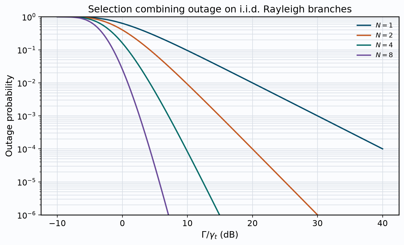
Figure 1 shows the point. Moving from one antenna to two drops the outage sharply; each added antenna multiplies the outage by another factor smaller than one. That is reliability bought with switches rather than with extra RF chains.

Sample simulation

import numpy as np
import matplotlib.pyplot as plt

ratio_db = np.linspace(-10, 40, 201)
ratio = 10 ** (ratio_db / 10)  # Gamma / gamma_t
plt.figure(figsize=(7.5, 4.5))
for N in (1, 2, 4, 8):
    pout = (1 - np.exp(-1.0 / ratio)) ** N
    plt.semilogy(ratio_db, pout, label="N=%d" % N)
plt.xlabel("Gamma/gamma_t (dB)"); plt.ylabel("Outage probability")
plt.ylim(1e-6, 1); plt.grid(True, which="both"); plt.legend(); plt.show()

Sample results

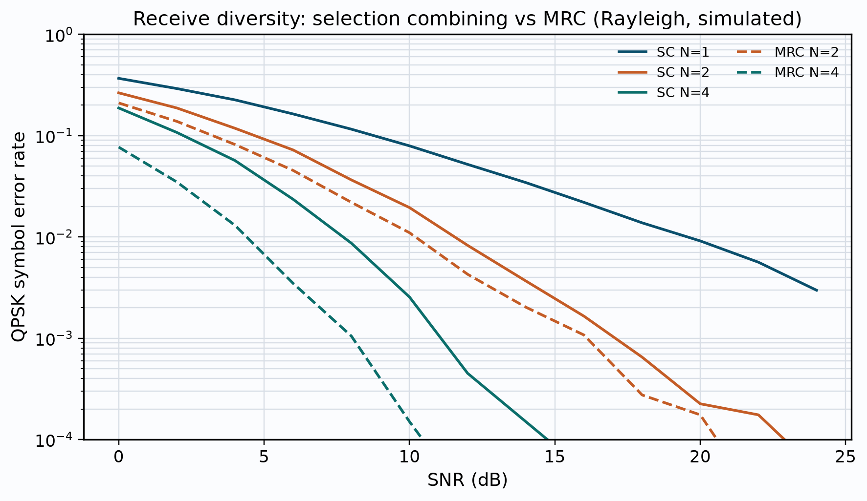
Figure 1 should match your plot. At an outage of \(10^{-4}\), the SNR saving from \(N=1\) to \(N=2\) is on the order of 20 dB on this normalised axis. Figure 2 already hints that MRC will do better for SER; SC remains the lower-complexity reference.

Next topic

Keep every branch and weight it optimally: maximum ratio combining.

References

1. M. K. Simon and M.-S. Alouini, Digital Communication over Fading Channels, 2nd ed., John Wiley & Sons, Hoboken, NJ, 2005.
2. A. Goldsmith, Wireless Communications, Cambridge University Press, Cambridge, UK, 2005.
3. D. G. Brennan, “Linear diversity combining techniques,” Proceedings of the IRE, vol. 47, no. 6, pp. 1075–1102, June 1959.
4. J. R. Barry, E. A. Lee, and D. G. Messerschmitt, Digital Communication, 3rd ed., Springer, New York, NY, 2004.

Frequently asked questions

How does selection combining decide which antenna to use? It measures the instantaneous SNR (or a proxy such as received power) on each branch and keeps only the strongest. After the switch, a single RF chain and demodulator process that branch; the other antennas contribute nothing to the decision statistic for that symbol.

What is the outage probability of selection combining on i.i.d. Rayleigh branches? If each branch SNR is exponential with mean \(\Gamma\), the combiner output is the maximum of the branch SNRs and \(P(\gamma_{\mathrm{out}}<\gamma_t)=(1-e^{-\gamma_t/\Gamma})^N\). At large average SNR this behaves as \((\gamma_t/\Gamma)^N\), so the diversity order is \(N\).

Why does selection combining achieve full diversity order yet lag MRC? The diversity order is set by the probability that all branches fade together, which still falls as \(\mathrm{SNR}^{-N}\). The coding gain is weaker than MRC’s because unused branches add no energy to the output SNR. MRC therefore reaches the same outage target at a lower average SNR.

When is selection combining preferred over MRC in practice? When RF-chain cost, power, or complexity dominate: after a switch you need only one down-conversion path. It is also a clean baseline against which soft combiners must justify their extra channel estimation and weighting hardware.