
MIMO — Diversity path
1. Intro → 2. Diversity vs mux → 3. SIMO → 4. Selection combining → 5. MRC
Introduction
Maximum ratio combining is the scheme Brennan analysed in 1959 and that textbooks still start from: co-phase the branches, weight them by amplitude, and add. Among linear combiners it maximises instantaneous SNR. Once you know MRC, selection combining looks like a deliberate simplification.
Motive
We want the best reliability a set of receive antennas can offer without yet introducing space-time codes. MRC uses every observation and needs channel estimates on each branch—the same CSI a coherent demodulator wants anyway. How much SNR and outage does that CSI buy?
Technical development
Set \(\mathbf{w}=\mathbf{h}\). Then
\[y=\sum_{k=1}^{N}h_k^\ast r_k, \qquad \gamma_{\mathrm{out}}=\sum_{k=1}^{N}\gamma_k.\]For i.i.d. Rayleigh branches the sum of exponential SNRs is Gamma-distributed with shape \(N\), and the outage probability is
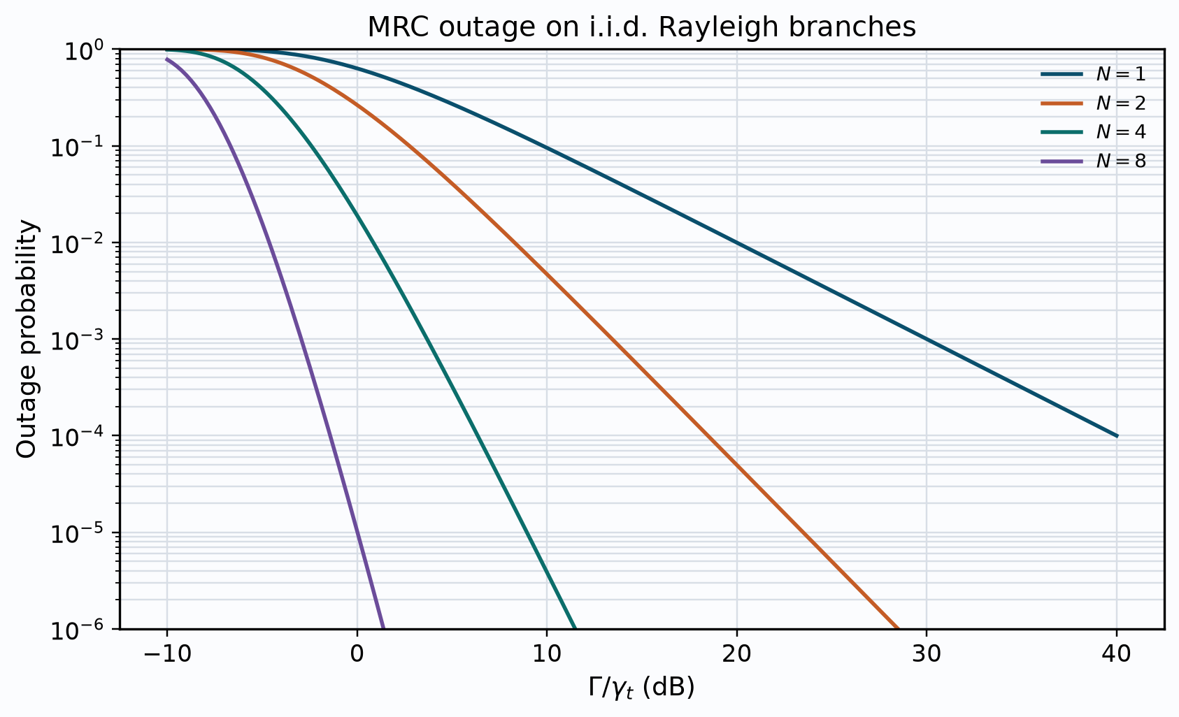
\[P_{\mathrm{out}}=1-e^{-\gamma_t/\Gamma}\sum_{n=0}^{N-1}\frac{(\gamma_t/\Gamma)^n}{n!}.\]Asymptotically this is still order \(N\), but the coding gain beats SC because every branch contributes.
How this achieves the motive
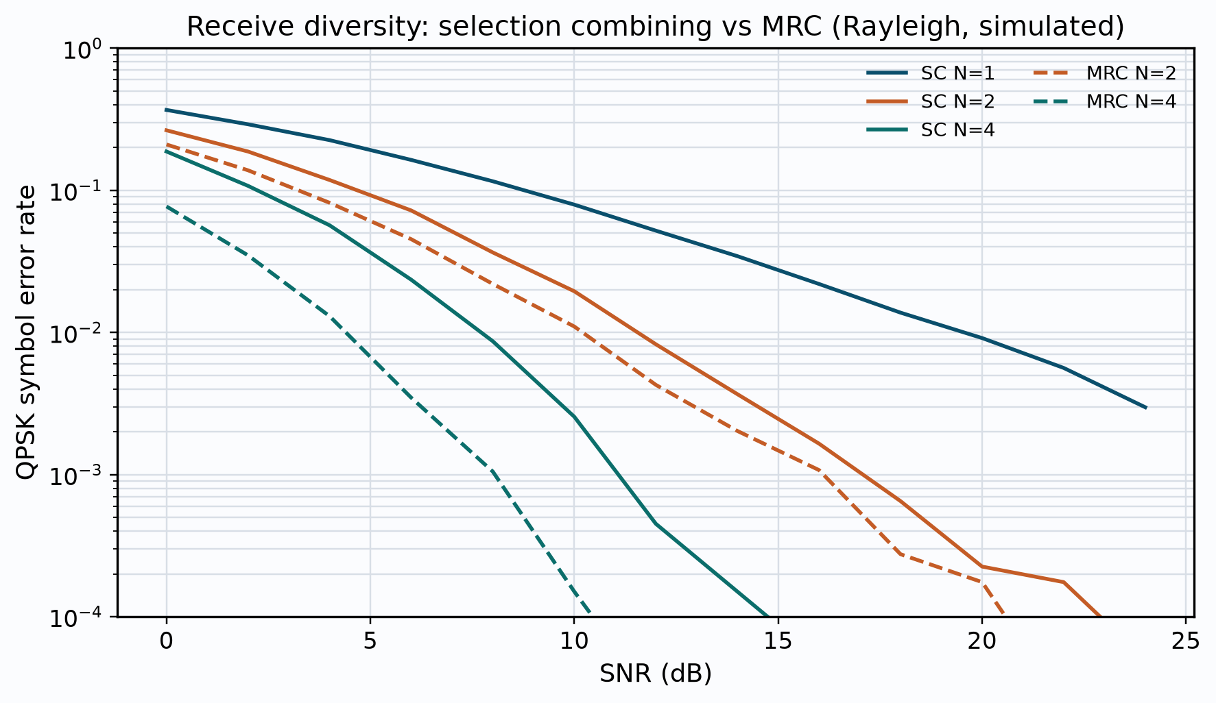
Compare Figure 1 with the SC outage plot in the previous article. Same diversity slopes, better horizontal position: MRC reaches a target outage at lower average SNR. The SER simulation in Figure 2 tells the same story for uncoded QPSK.
Sample simulation
import numpy as np
import matplotlib.pyplot as plt

ratio_db = np.linspace(-10, 40, 201)
x = 1.0 / (10 ** (ratio_db / 10))  # gamma_t / Gamma
plt.figure(figsize=(7.5, 4.5))
for N in (1, 2, 4, 8):
    s = np.zeros_like(x)
    term = np.ones_like(x)
    for k in range(N):
        if k:
            term = term * x / k
        s = s + term
    pout = 1 - np.exp(-x) * s
    plt.semilogy(ratio_db, np.maximum(pout, 1e-16), label="N=%d" % N)
plt.xlabel("Gamma/gamma_t (dB)"); plt.ylabel("Outage probability")
plt.ylim(1e-6, 1); plt.grid(True, which="both"); plt.legend(); plt.show()
Sample results
Your outage plot should reproduce Figure 1. On the SER figure, notice that MRC with \(N=2\) already rivals SC with a larger \(N\) over much of the SNR range—that is the gain from soft combining.
Next topic
That closes the diversity path. For rate and capacity, continue on the capacity path from channel modelling, or return to the multiple-antenna introduction.
References
- D. G. Brennan, “Linear diversity combining techniques,” Proceedings of the IRE, vol. 47, no. 6, pp. 1075–1102, June 1959.
- M. K. Simon and M.-S. Alouini, Digital Communication over Fading Channels, 2nd ed., John Wiley & Sons, Hoboken, NJ, 2005.
- A. Goldsmith, Wireless Communications, Cambridge University Press, Cambridge, UK, 2005.
- J. R. Barry, E. A. Lee, and D. G. Messerschmitt, Digital Communication, 3rd ed., Springer, New York, NY, 2004.
Frequently asked questions
How does maximum ratio combining form its decision statistic? With perfect CSI the weight vector equals the channel vector, \(\mathbf{w}=\mathbf{h}\). Each branch is co-phased and scaled by its amplitude, then the branches are summed. The instantaneous output SNR is the sum of the branch SNRs, which maximises SNR among all linear combiners.
What is the outage probability of MRC on i.i.d. Rayleigh branches? The sum of \(N\) independent exponential SNRs is Gamma-distributed with shape \(N\), and \(P_{\mathrm{out}}=1-e^{-\gamma_t/\Gamma}\sum_{n=0}^{N-1}(\gamma_t/\Gamma)^n/n!\). The diversity order remains \(N\), but the coding gain exceeds that of selection combining because every branch contributes.
Does MRC require more channel knowledge than selection combining? Yes. Selection combining needs only a ranking of branch strengths. MRC needs complex channel coefficients on every branch to set the phases and amplitudes correctly. The same CSI is typically already required for coherent demodulation.
Why is Brennan’s 1959 paper still cited for diversity combining? Brennan systematically compared selection, maximal-ratio, and equal-gain combining and derived the SNR relationships that textbooks still use. Modern MIMO receivers build on those linear-combining ideas before adding space-time coding and spatial multiplexing.