Diversity techniques and spatial multiplexing

In one sentence: Extra antennas can be spent in two ways — to make a link more reliable (diversity) or to make it faster (spatial multiplexing) — and this article shows how each works, what each buys you in dB and in bits per second per hertz, and how to choose between them.

A wireless channel fades. In a Rayleigh channel the instantaneous SNR of a single link is exponentially distributed, so a deep fade 10 dB below the mean happens roughly 10% of the time and a 20 dB fade about 1% of the time. A single-antenna receiver must therefore either waste power on a huge fade margin or accept frequent errors. Multiple antennas give us more than one propagation path to work with. The art is deciding what to do with them. Everything below assumes the standard textbook model: independent Rayleigh fading on each path, perfect channel knowledge at the receiver, and coherent detection.

1. Antenna configurations and notation

With $latex N_t$ transmit and $latex N_r$ receive antennas, the narrowband flat-fading link is $latex \mathbf{y} = \mathbf{H}\mathbf{x} + \mathbf{n}$, where $latex \mathbf{H}$ is an $latex N_r \times N_t$ matrix of complex path gains. The four classical configurations are:

• SISO — $latex N_t = N_r = 1$. One path, no spatial resource.
• SIMO — $latex N_t = 1,\ N_r > 1$. Receive diversity and array gain.
• MISO — $latex N_t > 1,\ N_r = 1$. Transmit diversity (for example Alamouti) or beamforming if the transmitter knows the channel.
• MIMO — $latex N_t > 1,\ N_r > 1$. Diversity, multiplexing, or a blend of the two.

With independent paths there are $latex N_t N_r$ distinct fading coefficients in $latex \mathbf{H}$. That product is the maximum diversity order. The number of independent data streams the matrix can carry is bounded by its rank, so the spatial degrees of freedom are at most $latex \min(N_t, N_r)$. Those are the two currencies of this article. Note that a SISO link has diversity order 1 (one path), not zero.

2. Four kinds of diversity

Diversity means sending, or receiving, the same information over several independently fading channels so that they are unlikely to all be bad at once. The channel can be made independent along four axes:

• Time diversity. Repeat or spread the information over intervals separated by more than the coherence time $latex T_c \approx 1/f_D$. Interleaving plus channel coding is the standard implementation. It fails for slow-moving users, because the channel never changes during the codeword.
• Frequency diversity. Use bandwidth wider than the coherence bandwidth $latex B_c \approx 1/\tau_{\mathrm{rms}}$ so different parts of the signal see different fades. Wideband CDMA with a rake receiver, and coded OFDM, harvest this. It needs a frequency-selective channel, which is bad news in a flat-fading environment.
• Space diversity. Use antennas spaced far enough apart (about half a wavelength or more, rich scattering assumed) that their fades are nearly uncorrelated. It costs no bandwidth and no extra time, only hardware and, at the transmitter, a split of the power budget.
• Polarization diversity. Use orthogonally polarized antennas at the same location. The scattering process tends to depolarize the wave, so the two polarizations fade independently. It is the cheapest option when there is no room for spacing, such as on a handset or a tower panel.

Space and polarization diversity are the ones that this article, and the rest of the Lab path, concentrate on, because they are the ones that scale with antenna count and do not consume bandwidth or latency.

3. Array gain versus diversity gain

Two different benefits get lumped together as “diversity”, and keeping them separate is the single most useful habit when you read a MIMO paper. At high average SNR $latex \bar\gamma$ the error rate of most schemes behaves like

$latex \displaystyle P_e \approx \left(G_a\,\bar\gamma\right)^{-G_d}$.

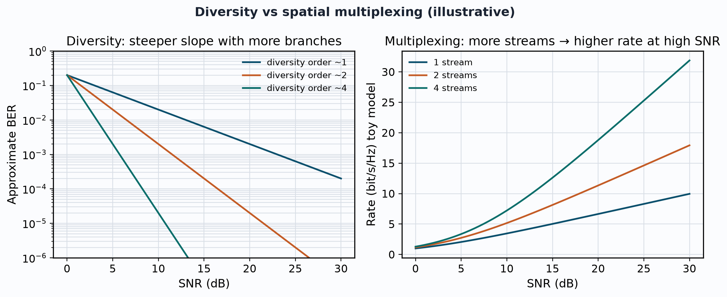
On a log-log BER plot, $latex G_d$ is the diversity gain (diversity order): the slope of the curve. $latex G_a$ is the array gain (coding or combining gain): a horizontal shift of the curve, measured in dB. Diversity gain fights fading; array gain fights noise.

Concretely, for coherent BPSK over Rayleigh fading with average SNR $latex \bar\gamma = E_b/N_0$ per branch, define $latex \mu = \sqrt{\bar\gamma/(1+\bar\gamma)}$. A single branch gives

$latex \displaystyle P_b = \tfrac{1}{2}\left(1-\mu\right) \;\approx\; \frac{1}{4\bar\gamma}$,

so the BER falls only one decade per 10 dB: diversity order 1. Compare AWGN, where the same SNR gives an exponentially small $latex Q(\sqrt{2\bar\gamma})$. Fading, not noise, is the problem. With $latex L$ independent branches combined optimally (MRC, Section 4):

$latex \displaystyle P_b = \left(\frac{1-\mu}{2}\right)^{\!L} \sum_{k=0}^{L-1} \binom{L-1+k}{k} \left(\frac{1+\mu}{2}\right)^{\!k} \;\approx\; \binom{2L-1}{L}\left(4\bar\gamma\right)^{-L}$.

The exponent $latex L$ is the diversity gain. The constant $latex \binom{2L-1}{L}4^{-L}$ plus the fact that MRC adds the branch SNRs (average output SNR $latex L\bar\gamma$) is where the array gain lives. A scheme can have a lot of one and none of the other: a single receive antenna with a very sensitive front end has array gain over a worse antenna but no diversity; selection among two uncorrelated antennas has diversity order 2 but little array gain.

4. Receive diversity at a glance

Take a SIMO link with $latex L$ receive branches and branch SNRs $latex \gamma_1,\dots,\gamma_L$, each exponentially distributed with mean $latex \bar\gamma$. The receiver combines the branches into one decision variable with output SNR $latex \gamma_{\mathrm{out}}$. Three combiners dominate textbooks:

• Selection combining (SC). Keep the strongest branch: $latex \gamma_{\mathrm{SC}} = \max_i \gamma_i$. Needs only an amplitude (power) measurement and one RF chain at a time. No phase information is required, so it even works with non-coherent detection.
• Equal-gain combining (EGC). Co-phase all branches and add them with equal weight: $latex \gamma_{\mathrm{EGC}} = \left(\sum_i \sqrt{\gamma_i}\right)^2 / L$. It needs the phase of each branch but not its amplitude.
• Maximum-ratio combining (MRC). Co-phase and weight each branch in proportion to its channel amplitude: $latex \gamma_{\mathrm{MRC}} = \sum_i \gamma_i$. It needs full channel knowledge and maximizes the output SNR for any set of channel gains.

All three reach full receive-diversity order $latex L$ in i.i.d. Rayleigh fading. They differ in array gain. In Rayleigh fading the mean output SNRs are

$latex \displaystyle \bar\gamma_{\mathrm{SC}} = \bar\gamma \sum_{k=1}^{L}\frac{1}{k}, \qquad \bar\gamma_{\mathrm{EGC}} = \bar\gamma\left[1+(L-1)\frac{\pi}{4}\right], \qquad \bar\gamma_{\mathrm{MRC}} = L\,\bar\gamma$.

For $latex L=2$ that is 1.76 dB (SC), 2.52 dB (EGC) and 3.01 dB (MRC) above one branch; for $latex L=4$ it is 3.19, 5.26 and 6.02 dB. The SC curve grows like $latex \ln L$, while MRC grows linearly in $latex L$ — one reason the returns on adding branches diminish under SC much faster than under MRC. The outage view says the same thing: for a threshold small compared with the average SNR, $latex t=\gamma_{\mathrm{th}}/\bar\gamma \ll 1$,

$latex \displaystyle P_{\mathrm{out}}^{\mathrm{SC}} = \left(1-e^{-t}\right)^L \approx t^{L}, \qquad P_{\mathrm{out}}^{\mathrm{MRC}} = 1-e^{-t}\sum_{k=0}^{L-1}\frac{t^k}{k!} \approx \frac{t^{L}}{L!}$.

Both curves have slope $latex L$ (diversity order $latex L$), but MRC sits lower by the constant factor $latex L!$ — array gain made visible. The numbers below are exact values at a target BER of $latex 10^{-3}$ for coherent BPSK in Rayleigh fading, from the same formulas the demo plots:

Scheme	$latex E_b/N_0$ needed for $latex 10^{-3}$	Gain vs one branch
1 branch	24.0 dB	—
SC, $latex L=2$	12.6 dB	11.4 dB
MRC, $latex L=2$	11.1 dB	12.9 dB
SC, $latex L=4$	7.3 dB	16.6 dB
MRC, $latex L=4$	4.0 dB	19.9 dB

Most of the benefit arrives with the second branch (about 11–13 dB), and each further branch adds less. The Lab path treats SC and MRC in full detail; the SIMO article sets up the signal model they share.

5. A short Monte-Carlo check of MRC

It is worth confirming the closed-form MRC expression against a simulation. The receiver forms $latex z = \mathrm{Re}\{\sum_i h_i^{*} y_i\}$, where $latex y_i = h_i s + w_i$, and decides on the sign of $latex z$. With unit-energy BPSK ($latex E_b = E_s = 1$) the complex noise variance is $latex 1/\gamma_b$, i.e. $latex \sigma^2 = 1/(E_b/N_0)$. See the Eb/N0, Es/N0 and SNR converter if the noise scaling is unfamiliar.

import numpy as np
from math import comb

def ber_mrc(L, snr_db):
    """Closed-form BPSK BER, L-branch MRC, i.i.d. Rayleigh."""
    g = 10 ** (snr_db / 10)
    mu = np.sqrt(g / (1 + g))
    p, q = (1 - mu) / 2, (1 + mu) / 2
    return p ** L * sum(comb(L - 1 + k, k) * q ** k for k in range(L))

def sim_mrc(L, snr_db, n=400_000, seed=1):
    rng = np.random.default_rng(seed)
    g = 10 ** (snr_db / 10)
    bits = rng.integers(0, 2, n)
    s = 1 - 2 * bits                                   # bit 0 -> +1
    h = (rng.standard_normal((L, n)) + 1j * rng.standard_normal((L, n))) / np.sqrt(2)
    w = (rng.standard_normal((L, n)) + 1j * rng.standard_normal((L, n))) / np.sqrt(2 * g)
    y = h * s + w
    z = np.sum(np.conj(h) * y, axis=0).real            # MRC decision variable
    return np.mean((z < 0).astype(int) != bits)

for L in (1, 2, 4):
    print(L, ber_mrc(L, 5), sim_mrc(L, 5))

At 5 dB the closed form gives about $latex 6.4\times10^{-2}$ ($latex L=1$), $latex 1.2\times10^{-2}$ ($latex L=2$) and $latex 5.1\times10^{-4}$ ($latex L=4$), and the simulation matches within sampling error. At higher SNR increase n so you still collect enough errors for a stable estimate.

6. Transmit diversity and the Alamouti scheme

Receive diversity is easy to explain but needs several antennas on the receiver, which is often the wrong side of the link (think of a phone). Transmit diversity moves the redundancy to the base station. The simplest and most famous scheme is Alamouti’s space-time block code for two transmit antennas. Over two symbol periods it sends

$latex \displaystyle \mathbf{X} = \begin{bmatrix} s_1 & -s_2^{*} \\ s_2 & s_1^{*} \end{bmatrix}$

(rows are antennas, columns are time slots). Because the two columns are orthogonal, a receiver that knows $latex h_1, h_2$ can decouple $latex s_1$ and $latex s_2$ with simple linear processing and obtain an effective SNR proportional to $latex |h_1|^2 + |h_2|^2$. The result is diversity order $latex 2N_r$ with $latex N_r$ receive antennas, at full rate (one symbol per channel use), with no channel knowledge at the transmitter. The price: the total transmit power is split across two antennas, so compared with a 1×2 MRC link the array gain is 3 dB lower. Diversity gain, not array gain, is what Alamouti delivers; beamforming with transmit channel knowledge is what recovers the array gain.

7. Spatial multiplexing: using the same antennas for rate

Diversity sends the same information over many paths. Spatial multiplexing sends different information. The transmitter splits the data into $latex S \le \min(N_t, N_r)$ parallel streams and transmits one per antenna in the same time and frequency resource. With rich scattering the matrix $latex \mathbf{H}$ has full rank, so the receiver can separate the streams. This is the BLAST family of architectures. Two things are remarkable: the rate multiplies by $latex S$ with no extra bandwidth, and, in the idealized model, no extra transmit power.

Separating the streams is a detection problem. Three standard receivers:

• Zero forcing (ZF) applies $latex \mathbf{H}^{\dagger}$ (the pseudo-inverse) and completely removes inter-stream interference, at the price of amplifying noise when $latex \mathbf{H}$ is ill-conditioned. Needs $latex N_r \ge S$. Diversity order per stream: $latex N_r - S + 1$.
• MMSE trades a little residual interference for much less noise enhancement. Same diversity order as ZF, but better at low SNR.
• Maximum likelihood (ML) searches all constellation vectors. It reaches diversity order $latex N_r$, but its complexity grows exponentially with the number of streams (sphere decoding reduces that).

Notice the catch: pushing the receiver to separate $latex S$ streams spends receive degrees of freedom. A 2×2 link with ZF detection has diversity order $latex 2-2+1 = 1$ — no better than SISO, despite having four fading coefficients. The antennas have been traded for rate.

8. MIMO capacity intuition

For an i.i.d. Rayleigh channel with perfect receiver knowledge and equal power on each transmit antenna (no transmit channel knowledge), the ergodic capacity is

$latex \displaystyle C = \mathbb{E}\left[\log_2 \det\!\left(\mathbf{I}_{N_r} + \frac{\rho}{N_t}\mathbf{H}\mathbf{H}^{H}\right)\right] \quad \text{bit/s/Hz}$,

where $latex \rho$ is the average SNR at each receive antenna. Two limits give the picture.

• High SNR: $latex C \approx \min(N_t,N_r)\,\log_2\rho + \text{const}$. The curve is as if the channel were $latex \min(N_t,N_r)$ parallel SISO channels. Each 3 dB of SNR buys $latex \min(N_t,N_r)$ extra bit/s/Hz instead of 1. This slope is the “multiplexing gain”.
• Low SNR: $latex C \approx N_r\,\rho\,\log_2 e$. Capacity is limited by received power, so extra receive antennas help through array gain and extra streams do not.

Numbers make this concrete. Monte-Carlo averages over 1000 channel draws, with the SISO value computed exactly, give:

Configuration	10 dB	20 dB
SISO 1×1	2.91	5.88
MISO 4×1 (no transmit CSI)	3.3	6.5
SIMO 1×4	5.2	8.4
MIMO 2×2	5.6	11.3
MIMO 4×4	11.0	22.2

Values are in bit/s/Hz. SIMO 1×4 adds array gain: it lifts the curve by roughly 2.3–2.6 bit/s/Hz at both SNRs but does not change the slope. MISO 4×1 without channel knowledge gets almost nothing. Only the MIMO links with several streams multiply the slope (2×2 doubles it, 4×4 quadruples it): the 4×4 link carries about 3.8 times SISO at 20 dB. Capacity says nothing about how reliable a particular scheme is at a given rate. For that we need the next section.

9. The diversity–multiplexing trade-off

Sections 3–8 treated diversity and multiplexing as separate options. In reality a scheme that is asked to carry a higher rate has less room to protect itself against fades. Zheng and Tse formalized this: if the data rate scales as $latex R = r\log_2\rho$ with multiplexing gain $latex r$, the best error probability achievable behaves like $latex \rho^{-d^{*}(r)}$, where $latex d^{*}(r)$ is the piecewise-linear function joining the points

$latex \displaystyle \bigl(k,\ (N_t-k)(N_r-k)\bigr), \qquad k = 0,1,\dots,\min(N_t,N_r)$.

Two ends of the curve recover everything we have already seen. At $latex r=0$ (fixed rate) the diversity order is the maximum $latex N_tN_r$. At $latex r=\min(N_t,N_r)$ (all streams, full multiplexing) the diversity is zero: the data rate grows as fast as capacity, and there is no reliability to spare. A 2×2 link goes through $latex (0,4)$, $latex (1,1)$ and $latex (2,0)$. Look at the middle point: running one stream of multiplexing gain already cuts the available diversity from 4 to 1.

The frontier is a bound, not a scheme. Practical designs sit below it: MRC and ML spatial multiplexing give diversity $latex N_r$ at fixed rate; Alamouti gives $latex 2N_r$; full-rank space-time codes aim for $latex N_tN_r$. Open the 2×2 frontier in the demo and move to 4×4 to see how a larger array gives the designer more room in both directions.

10. When to use which

There is no universally best choice; the right one depends on SNR, scattering, and what the transmitter knows.

Situation	Prefer	Why
Low SNR, cell edge, power-limited link	Diversity or beamforming	Capacity is power-limited; extra streams would have almost no SNR each.
High SNR, rich scattering, throughput target	Spatial multiplexing	Capacity slope scales with $latex \min(N_t,N_r)$; reliability margin is cheap at high SNR.
Strict reliability, short packets, no retransmission	Diversity (Alamouti, MRC)	Pushes the BER slope up, removing the need for a large fade margin.
Transmitter has no channel knowledge	Alamouti, open-loop multiplexing	Neither scheme needs feedback about $latex \mathbf{H}$.
Transmitter has good channel knowledge	Beamforming and precoded multiplexing	Feedback recovers array gain and lets streams be matched to the strongest eigenmodes.
Correlated antennas, line-of-sight, high Rician K	Beamforming, one stream	Channel rank is low; the streams you would multiplex are not independent.

Modern standards do not pick once and for all. LTE and 5G NR adapt per link: when the reported channel quality is poor or the channel is nearly rank one, the scheduler uses transmit diversity (Alamouti-style space-frequency block coding in LTE) or a single beamformed stream; when quality is high and the channel supports it, it increases the rank and sends more layers. Selecting the number of streams is, in the language of Section 9, choosing a point on the diversity–multiplexing frontier for the instantaneous channel.

11. Try it yourself

The Diversity vs spatial multiplexing demo implements the formulas of Sections 3, 4, 8 and 9. In Lab A, sweep $latex L$ from 2 to 8 and compare single-branch, SC and MRC curves, or switch to the outage view to read the fade margin you save. In Lab B, move the antenna counts and watch the diversity–multiplexing frontier and the capacity curves change. Every setting is in the URL, so you can share a configuration.

FAQ

What is the difference between diversity gain and array gain? Diversity gain is the slope of the error-rate curve (the exponent $latex G_d$ in $latex P_e \approx (G_a\bar\gamma)^{-G_d}$); it measures how well fading is averaged out. Array gain is a horizontal shift in dB of that same curve; it measures how much extra signal power the combiner collects. SC has diversity order $latex L$ but little array gain; MRC has both.

Is MRC always better than selection combining? For SNR it is: $latex \sum_i\gamma_i \ge \max_i\gamma_i$ for every channel realization. The trade is cost: MRC needs a full RF chain and channel estimate for every branch, whereas SC needs one RF chain at a time and only a power measurement. Whether the extra 1–3 dB at $latex L=2\text{ to }4$ matters depends on the link budget.

Can a MIMO system get full diversity and full multiplexing simultaneously? No. The Zheng–Tse frontier shows that at the maximum multiplexing gain $latex \min(N_t,N_r)$ the diversity gain drops to zero, and at maximum diversity $latex N_tN_r$ the multiplexing gain is zero. Every other operating point lies on the line segments between them.

Why does a 2×2 spatial-multiplexing link not have diversity order 4? Four fading coefficients exist, but separating two streams with a linear receiver consumes receive degrees of freedom. ZF leaves $latex N_r-S+1 = 1$ order per stream, and even ML detection reaches only $latex N_r = 2$. Only a code that spreads each symbol over both antennas and both time slots (such as Alamouti for a single stream) can use all four paths.

How far apart must antennas be for space diversity to work? There is no sharp threshold. A spacing of about half a wavelength gives low correlation in rich-scattering environments at the mobile; base stations, which see a narrow angular spread, often need many wavelengths (or use polarization diversity). Correlation reduces the diversity order toward 1 and the capacity slope toward that of SISO.

Does diversity help in AWGN-only channels? It still adds array gain (combining noisy copies raises SNR), but there are no fades to average out, so the error curve keeps its AWGN slope — as the dotted AWGN curve in the demo shows, diversity combining in Rayleigh fading approaches that curve as $latex L$ grows.

Similar articles

• Introduction to multiple antenna systems
• Characterizing a MIMO channel
• SIMO models for receive diversity
• Receiver diversity: selection combining
• Receiver diversity: maximum ratio combining (MRC)
• MIMO: an overview of multi-input multi-output technology
• Diversity vs spatial multiplexing demo