Hard vs soft decision decoding — bits, metrics, and coding gain

Imagine you are a judge in a courtroom listening to a witness:

• Hard Decision: The witness is only allowed to answer “Yes” or “No”. Even if they are $51\%$ sure, they must commit to a hard “Yes”.
• Soft Decision: The witness can say “I am 51% sure it was Yes” or “I am 99% sure it was Yes”.

In digital communications, noise corrupts electrical signals as they travel through the air or cables. Soft decision decoding keeps that extra percentage of certainty, whereas hard decision throws it away.

Step 1: Setting Up the Encoder

Before transmitting digital bits ($0$s and $1$s), a transmitter adds extra check bits called parity bits to help detect or fix errors.

Suppose we want to send a $2$-bit message: 01.

We add a $3\text{rd}$ bit (a parity bit) so that the total count of $1$s in the $3$-bit combination is always an even number:

Message Bits	Parity Bit Added	Generated Codeword	Total 1s Count
00	0	000	$0$ (Even)
01	1	011	$2$ (Even)
10	1	101	$2$ (Even)
11	0	110	$2$ (Even)

The set of valid $3$-bit codewords that the receiver knows about are: 000, 011, 101, and 110.

We convert these bits into voltages: $0 = 0\text{ Volts}$ and $1 = 1\text{ Volt}$. We transmit the message 01, which corresponds to codeword 011 ($0\text{V}, 1\text{V}, 1\text{V}$).

Step 2: Channel Distortion

As the signal travels over the noisy channel, noise pushes the voltages around. At the receiver, instead of seeing clean $0\text{V}$ and $1\text{V}$, we sample three corrupted voltages:

$$\text{Received Voltages} = (0.2\text{V}, \quad 0.4\text{V}, \quad 0.7\text{V})$$

Now, let me show you how a Hard Decision Receiver vs. a Soft Decision Receiver handles these three measurements.

Step 3: Method 1 — Hard Decision Decoding

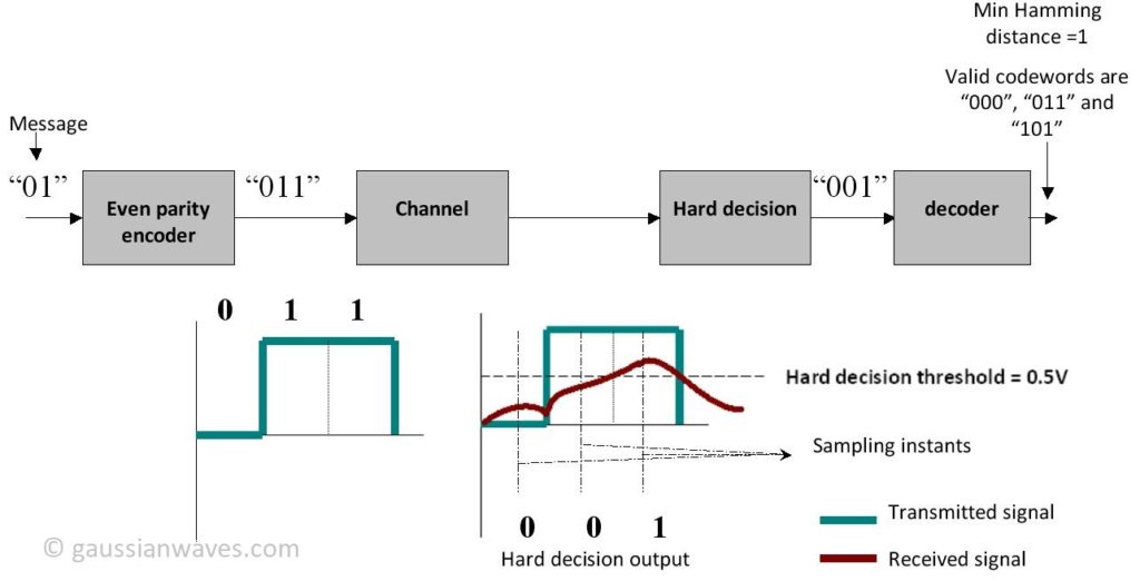
A hard decision decoder uses a rigid threshold midway between $0\text{V}$ and $1\text{V}$ ($0.5\text{V}$):

• If Voltage $< 0.5\text{V} \rightarrow$ decide bit is 0
• If Voltage $\ge 0.5\text{V} \rightarrow$ decide bit is 1

Let’s slice our received voltages $(0.2\text{V}, 0.4\text{V}, 0.7\text{V})$:

1. $0.2\text{V} < 0.5\text{V} \rightarrow$0
2. $0.4\text{V} < 0.5\text{V} \rightarrow$0(Notice: $0.4\text{V}$ was very close to $0.5\text{V}$, but it gets forced into a 0 anyway!)
3. $0.7\text{V} \ge 0.5\text{V} \rightarrow$1

The hard decision block outputs the bit sequence: 001.

Finding the Closest Match (Hamming Distance)

Hamming Distance simply counts how many bit positions differ between two sequences. The decoder compares 001 against all valid codewords:

Valid Codeword	Hard Decision Output	Differing Bit Positions	Hamming Distance
000	001	$3\text{rd}$ bit	1
011	001	$2\text{nd}$ bit	1
101	001	$1\text{st}$ bit	1
110	001	All bits	3

The Problem: Three valid codewords (000, 011, 101) tie with a minimum Hamming distance of $1$. The decoder has no idea which one was actually sent and must guess randomly. The chance of guessing the right one (011) is only $\frac{1}{3}$ ($33.3\%$).

Step 4: Method 2 — Soft Decision Decoding

A soft decision decoder refuses to slice the voltage into $0$s and $1$s early. Instead, it measures the physical “distance” between the raw received voltages $(0.2\text{V}, 0.4\text{V}, 0.7\text{V})$ and the target voltages of every valid codeword using Euclidean Distance.

What is Euclidean Distance?

It is simply the standard geometry equation for distance between points:

$$D^2 = (V_{1, \text{ideal}} – V_{1, \text{received}})^2 + (V_{2, \text{ideal}} – V_{2, \text{received}})^2 + (V_{3, \text{ideal}} – V_{3, \text{received}})^2$$

Let’s calculate $D^2$ for each candidate codeword:

1. For Codeword 000 ($0\text{V}, 0\text{V}, 0\text{V}$):
   $$D^2 = (0 – 0.2)^2 + (0 – 0.4)^2 + (0 – 0.7)^2 = 0.04 + 0.16 + 0.49 = \mathbf{0.69}$$
2. For Codeword 011 ($0\text{V}, 1\text{V}, 1\text{V}$):
   $$D^2 = (0 – 0.2)^2 + (1 – 0.4)^2 + (1 – 0.7)^2 = 0.04 + 0.36 + 0.09 = \mathbf{0.49}$$
3. For Codeword 101 ($1\text{V}, 0\text{V}, 1\text{V}$):
   $$D^2 = (1 – 0.2)^2 + (0 – 0.4)^2 + (1 – 0.7)^2 = 0.64 + 0.16 + 0.09 = \mathbf{0.89}$$
4. For Codeword 110 ($1\text{V}, 1\text{V}, 0\text{V}$):
   $$D^2 = (1 – 0.2)^2 + (1 – 0.4)^2 + (0 – 0.7)^2 = 0.64 + 0.36 + 0.49 = \mathbf{1.49}$$

Step 5: The Verdict

Valid Codeword	Distance Metric Used	Distance Score	Result
000	Euclidean Distance	$0.69$	Runner-up
011	Euclidean Distance	$0.49$	Winner (Smallest Distance)
101	Euclidean Distance	$0.89$	—
110	Euclidean Distance	$1.49$	—

The soft decision decoder uniquely picks 011—recovering the exact message sent with $100\%$ accuracy!

Why Did Soft Decoding Win?

When the second voltage arrived as $0.4\text{V}$:

• Hard Decision threw away information by declaring $0.4\text{V} < 0.5\text{V} \rightarrow 0$ with equal confidence as if it were $0.0\text{V}$.
• Soft Decision recognized that $0.4\text{V}$ was much closer to $1\text{V}$ than $0.7\text{V}$ was to $0\text{V}$. By preserving that raw voltage magnitude, it allowed the overall energy calculation to point decisively to the correct answer.

Modern Soft Decoding: Log-Likelihood Ratios (LLRs)

In modern receivers, decoders rarely process raw voltage levels or simple binary digits ($0$ and $1$). Instead, the demodulator passes continuous probabilistic values called Log-Likelihood Ratios (LLRs).

What is a Log-Likelihood Ratio?

An LLR condenses two pieces of vital information into a single number:

1. The Sign ($\pm$): Indicates the most likely transmitted bit ($0$ or $1$).
2. The Magnitude ($\vert{}L\vert{}$): Indicates the receiver’s confidence in that decision.

Mathematically, for a received noisy voltage $y$, the LLR is the natural logarithm of the ratio of probabilities:

$$L(y) = \ln \left( \frac{P(b=0 \mid y)}{P(b=1 \mid y)} \right)$$

If we transmit $0$ as $0\text{ V}$ and $1$ as $1\text{ V}$ over a channel with Gaussian noise variance $\sigma^2$ (assuming equal prior probabilities for $0$ and $1$), this probability ratio reduces to:

$$L(y) = \frac{1 – 2y}{2\sigma^2}$$

How to Read This Formula:

• Effect of Voltage ($y$):
  • If $y = 0.2\text{ V}$ (closer to $0\text{ V}$), $1 – 2(0.2) = +0.6 > 0$. A positive sign favors bit 0.
  • If $y = 0.7\text{ V}$ (closer to $1\text{ V}$), $1 – 2(0.7) = -0.4 < 0$. A negative sign favors bit 1.
• Effect of Noise ($\sigma^2$):
  • The noise variance $\sigma^2$ sits in the denominator. When channel noise is low ($\sigma^2$ is small), $L(y)$ becomes very large—reflecting high confidence. When noise is high ($\sigma^2$ is large), $L(y)$ shrinks toward zero—reflecting uncertainty.

Antipodal Mapping (The Standard in Real Systems)

In wireless standards (like BPSK), bits are mapped symmetrically: $0 \rightarrow +1\text{ V}$ and $1 \rightarrow -1\text{ V}$. Under this antipodal mapping, the LLR formula becomes even simpler:

$$L(y) = \frac{2y}{\sigma^2}$$

Here, a positive received voltage $y$ directly yields a positive LLR (favoring bit 0), and a negative voltage yields a negative LLR (favoring bit 1).

Python Verification Script

Here is a simple Python script using numpy to recompute the Hamming distances, Euclidean distances, and LLRs from our example:

import numpy as np

# 1. Define valid 3-bit codewords for our parity encoder
codewords = np.array([
    [0, 0, 0],
    [0, 1, 1],
    [1, 0, 1],
    [1, 1, 0],
], dtype=float)

# 2. Define received hard-sliced bits and soft continuous voltages
hard = np.array([0, 0, 1])
soft = np.array([0.2, 0.4, 0.7])

# 3. Calculate distance metrics
hamming = np.sum(codewords != hard, axis=1).astype(int)
euclidean = np.sum((codewords - soft) ** 2, axis=1)

print("Hamming Distances:          ", hamming.tolist())
print("Euclidean Distances:        ", np.round(euclidean, 2).tolist())
print("Hard-decision tied candidates:", codewords[hamming == hamming.min()].astype(int).tolist())
print("Soft-decision winning codeword:", codewords[np.argmin(euclidean)].astype(int).tolist())

# 4. Compute Log-Likelihood Ratios (LLRs) for noise variance sigma^2 = 0.25
sigma2 = 0.25
llr = (1.0 - 2.0 * soft) / (2.0 * sigma2)
print("LLRs (Positive favors 0):    ", np.round(llr, 3).tolist())

Sample output

Hamming Distances: [1, 1, 1, 3]
Euclidean Distances: [0.69, 0.49, 0.89, 1.49]
Hard-decision tied candidates: [[0, 0, 0], [0, 1, 1], [1, 0, 1]]
Soft-decision winning codeword: [0, 1, 1]
LLRs (Positive favors 0): [1.2, 0.4, -0.8]

• Hamming Distances:[1, 1, 1, 3]$\rightarrow$ Hard decision produces a 3-way tie (000, 011, 101).
• Euclidean Distances:[0.69, 0.49, 0.89, 1.49]$\rightarrow$ Minimum distance is $0.49$, corresponding uniquely to 011 (the correct message).
• Calculated LLRs:[1.2, 0.4, -0.8]
  • $0.2\text{ V} \rightarrow \text{LLR} = +1.2$ (Strong confidence for 0)
  • $0.4\text{ V} \rightarrow \text{LLR} = +0.4$ (Weak confidence for 0)
  • $0.7\text{ V} \rightarrow \text{LLR} = -0.8$ (Moderate confidence for 1)

Key Takeaways & A Warning

1. Information Loss: Hard decision decoders discards valuable signal magnitude information during early threshold slicing. Soft decision decoders retain this analog uncertainty throughout the decoding process.
2. A Note on Parity Codes: Our simple $3$-bit parity code is an example used to illustrate the concept. Simple parity codes can only detect single-bit errors; they are not powerful enough to reliably correct errors under all noise patterns (e.g., if received voltages were $0.2\text{ V}, 0.4\text{ V}, 0.6\text{ V}$, soft decoding would pick 000 instead of 011).
3. Where Soft Decision Really Shines: The power of soft decision decoding becomes transformative when paired with robust Forward Error Correction (FEC) codes—such as Convolutional Codes, Turbo Codes, and LDPC (Low-Density Parity-Check) codes used in $5\text{G}$ and Wi-Fi.

Soft Decoding in Practice: Viterbi & SOVA

In sequence estimation over a trellis (such as Viterbi decoding for convolutional codes):

The Soft-Output Viterbi Algorithm (SOVA)—introduced by Hagenauer and Hoeher in 1989—goes one step further: it outputs both the decided bit and a reliability value for that bit. This reliability output is critical in concatenated coding schemes (like Turbo codes), where one decoder’s soft output becomes the next decoder’s soft input.

A Soft-Input Viterbi Decoder uses Euclidean distances (or LLR branch metrics) to track the most likely path through a state diagram. At the very end, it outputs hard bits ($0$ or $1$).

For further reading

[1] J. Hagenauer and P. Hoeher, “A Viterbi algorithm with soft-decision outputs and its applications,” IEEE GLOBECOM, pp. 1680–1686, 1989.
[2] S. Lin and D. J. Costello, Error Control Coding, 2nd ed., Pearson, 2004, Chapter 10.

FAQ

What is a soft decision value in a decoder? Instead of passing a hard 0/1 bit, the demodulator passes a real-valued reliability, commonly a log-likelihood ratio (LLR). The sign is the bit guess; the magnitude says how confident the channel observation was.

Why does soft-decision decoding usually gain about 2 dB? Hard decisions throw away amplitude information, so the decoder treats every bit flip as equally likely. Soft metrics let the decoder down-weight unreliable bits and perform closer to true maximum-likelihood sequence detection on the code trellis or graph.

When is hard decision still acceptable? At very high SNR, for extremely simple parity checks, or when implementation cost forbids LLRs. Otherwise, modern links (LTE/NR turbo/LDPC, Wi-Fi LDPC, etc.) expect soft inputs.