
Detection path:
ML estimation →
ML decoding →
Hard vs soft decision →
Hamming codes
In one sentence: Maximum-likelihood decoding picks the codeword that maximizes the channel likelihood of the received word — on a BSC that reduces to nearest Hamming neighbor when the crossover probability is below one half.
Introduction
Maximum likelihood decoding is a technique used to determine the most likely transmitted message in a digital communication system, based on the received signal and statistical models of noise and interference. The method uses maximum likelihood estimation to calculate the probability of each possible transmitted message and then selects the one with the highest probability.
To perform maximum likelihood decoding, the receiver uses a set of pre-defined models to estimate the likelihood of each possible transmitted message based on the received signal. The method is commonly used in various digital communication and data storage systems, such as wireless communication and digital storage. However, it can be complex and time-consuming, particularly in systems with large message spaces or complex noise and interference models.
Maximum Likelihood Decoding:
Consider a set of possible codewords (valid codewords – set \(Y\)) generated by an encoder in the transmitter side. We pick one codeword out of this set ( call it \(y\) ) and transmit it via a Binary Symmetric Channel (BSC) with probability of error \(p\) ( To know what is a BSC –binary symmetric channel). At the receiver side we receive the distorted version of \(y\) ( call this erroneous codeword \(x\)).
Maximum likelihood decoding chooses the codeword \(y\) that maximizes the likelihood of what was received. With \(y\) the transmitted codeword and \(x\) the received word, that probability is
\[\mathbb{P}(x\;\text{received}\mid y\;\text{sent})\]Maximizing \(P(y\,\text{sent}\mid x\,\text{received})\) is maximum a posteriori (MAP) decoding. When every codeword is equally likely the prior is a constant, Bayes’ rule says the two rules pick the same codeword, and the distinction is easy to miss. They part company as soon as the codewords are not equally likely. The rest of this article assumes they are, so the ML rule is the one to compute.
The receiver knows \(x\) and does not know \(y\). It evaluates the likelihood for every codeword in the book and keeps the largest. That search is not a parameter estimate. Maximum likelihood estimation, the subject of the companion article, fits an unknown number such as a crossover probability. Decoding treats the channel law as known and chooses a message.
Examples for “Prediction” and “Estimation” :
1) Probability of getting a “Head” in a single toss of a fair coin is \(0.5\). The coin is tossed 100 times in a row.Prediction helps in predicting the outcome ( head or tail ) of the \(101^{th}\) toss based on the probability.
2) A coin is tossed 100 times and the data ( head or tail information) is recorded. Assuming the event follows Binomial distribution model, estimation helps in determining the probability of the event. The actual probability may or may not be \(0.5\). Maximum Likelihood Estimation estimates the conditional probability based on the observed data ( received data – \(x\)) and an assumed model.
Example of Maximum Likelihood Decoding:
Let \(y=11001001\) and \(x=10011001\) . Assuming Binomial distribution model for the event with probability of error \(0.1\) (i.e the reliability of the BSC is \(1-p = 0.9\)), the Hamming distance between codewords is \(2\) . For binomial model,
\[\mathbb{P}(x\;\text{received}\mid y\;\text{sent}) = (1-p)^{n-d}\, p^{d}\]where \(d\) is the Hamming distance between the sent codeword and the received word, \(n\) is the number of bits in the word, and \(p\) is the crossover probability of the BSC. The factor \(1-p\) is the probability that a given bit arrives intact.
With \(d=2\), \(n=8\) and \(p=0.1\), the likelihood of this particular pair is \((0.9)^{6}(0.1)^{2} = 0.005314\). A decoder still has to compare that number with the likelihood of every other codeword. For any \(p < 1/2\) the expression \((1-p)^{n-d}p^{d}\) falls as \(d\) grows, so the comparison reduces to finding the codeword closest to \(x\) in Hamming distance. The numerical value of \(p\) is not required, only the knowledge that it sits below one half.
Hamming distance is the ML metric on the BSC. Euclidean distance is the ML metric for soft samples in AWGN, where the likelihood is a Gaussian density in the analog vector. The two distances belong to two different channel laws. Using one in place of the other changes the decoder.
In practice \(y\) is not known at the receiver. The binomial expression is still the right likelihood: it is evaluated for every codeword in the book, and the largest one is kept.
Since the receiver is unaware of the particular \(y\) corresponding to the \(x\) received, the receiver computes \(P(y\; received \mid x\; sent)\) for each codeword in \(Y\). The \(y\) which gives the maximum probability is concluded as the codeword that was sent.
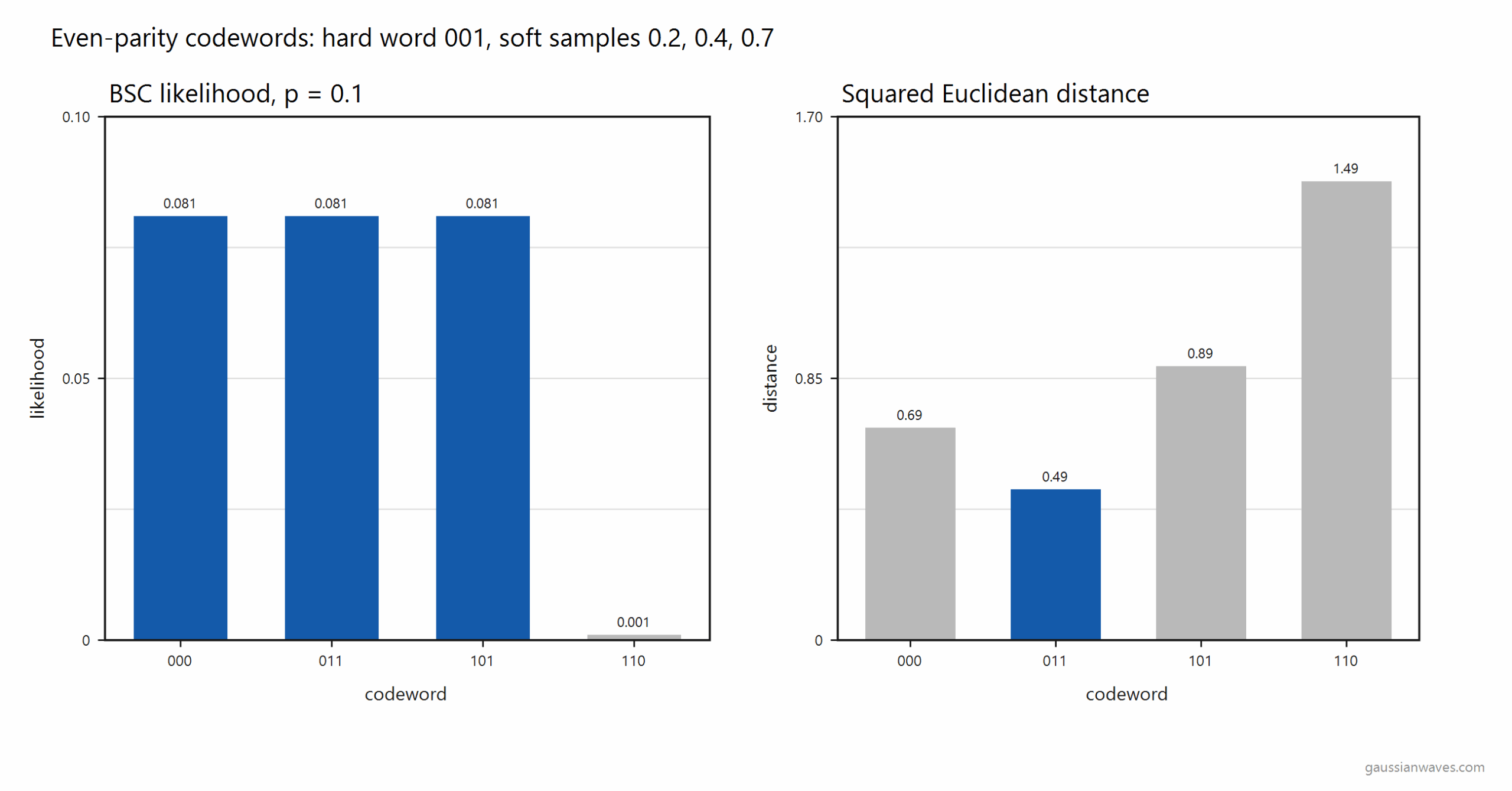
The listing decodes a small even-parity book on a BSC, which is the problem set up above, and then repeats the same book with soft samples so the Euclidean rule is visible beside the Hamming rule. The received hard word is 001 and the transmitted word is 011, the same numbers used in the hard and soft decision article. On the BSC the three codewords at distance 1 are tied. On the soft samples, 011 is the unique nearest codeword.
import numpy as np

codebook = np.array([
    [0, 0, 0],
    [0, 1, 1],
    [1, 0, 1],
    [1, 1, 0],
], dtype=int)
received_hard = np.array([0, 0, 1])
p = 0.1
n = received_hard.size
distance = np.sum(codebook != received_hard, axis=1)
likelihood = ((1 - p) ** (n - distance)) * (p ** distance)
print("Hamming distance", distance.tolist())
print("BSC likelihood ", np.round(likelihood, 6).tolist())
print("ML set", codebook[likelihood == likelihood.max()].tolist())

soft = np.array([0.2, 0.4, 0.7])
euclidean = np.sum((codebook - soft) ** 2, axis=1)
print("Euclidean", np.round(euclidean, 2).tolist())
print("Soft ML", codebook[np.argmin(euclidean)].tolist())
The figure puts both metrics on the four codewords. On the BSC the three words at distance 1 share the likelihood 0.081. The soft samples break that tie: the squared Euclidean distance selects 011.
Reference :
[1] Parameter fitting is the subject of the companion note on maximum likelihood estimation. Decoding, as above, treats the channel law as known.
FAQ
Is ML decoding the same as ML estimation? No. Estimation fits an unknown parameter (for example a crossover probability) from data. Decoding treats the channel law as known and chooses which message was sent. See the MLE companion article.
When does ML decoding become nearest-neighbor decoding? On a binary symmetric channel with crossover probability $latex p<1/2$, the likelihood $(1-p)^{n-d}p^{d}$ decreases with Hamming distance $latex d$, so maximizing likelihood is equivalent to minimizing Hamming distance.
What changes for soft AWGN samples? The ML metric becomes Euclidean distance (or a log-likelihood ratio for coded bits), not Hamming distance. Using the wrong metric for the channel law changes the decoder.
Similar articles
Related Topics:
Hello! Great explanation. It helped me a lot.
I wanted to tell you that I think there is a small mistake. One of your paragraphs begin with “In practice we don’t know Y (at the receiver) but we know x.” I think you mean ‘y’ (non capital) instead of ‘Y’. I think at the receiver we know Y, the set of all codewords. Later on, we can compute the hamming distances because we know this set. Isn’t this correct? Thanks for the explanation
Thank for catching the mistake. It is corrected now. Yes, the transmitter and receiver should agree on the set of codewords (the coding scheme) used. Receiver computes likelihood for all set of codewords and selects the one that maximizes the likelihood.