The Cramer Rao lower bound introduction starts with a simple question: how accurately can any unbiased estimator measure an unknown value? The Cramér-Rao lower bound (CRLB) gives a hard answer. It is a floor on the variance of every unbiased estimator, so it tells you what is achievable before you design anything. This post explains the idea with two worked examples and Python simulations that check the theory.
The problem: estimating a value from noisy data
An estimator is a rule that turns measured data into a guess at an unknown quantity. The quantity is called a parameter, written $\theta$. The guess is the estimate, written $\hat{\theta}$.
Two properties matter:
- Unbiased: on average the estimator hits the true value, $E\lbrace \hat{\theta}\rbrace = \theta$. Here $E\lbrace \cdot\rbrace $ means the average over many noisy datasets.
- Variance: how much the estimates scatter around their average, $\mathrm{var}(\hat{\theta}) = E\lbrace (\hat{\theta} – E\lbrace \hat{\theta}\rbrace )^2\rbrace $. A smaller variance means more precise estimates.
Among all unbiased estimators, the best one has the smallest variance. It is called the minimum variance unbiased estimator (MVUE). Checking that your estimator’s variance is small is easy. Checking that no other estimator does better is much harder. The CRLB answers that question.
The bound: a floor on the variance
Let $p(x;\theta)$ be the likelihood: the probability of the data $x$ for a given value of $\theta$. Two quantities come from it:
- The score is the slope of the log-likelihood with respect to $\theta$: $\dfrac{\partial \ln p(x;\theta)}{\partial \theta}$.
- The Fisher information measures how much the data reveal about $\theta$. It is the average squared score:
$$I(\theta) = E\left\lbrace \left(\frac{\partial \ln p(x;\theta)}{\partial \theta}\right)^2\right\rbrace $$
The Cramér-Rao bound says that, for any unbiased estimator $\hat{\theta}$ under mild smoothness conditions on $p(x;\theta)$,
$$\mathrm{var}(\hat{\theta}) \ \ge\ \frac{1}{I(\theta)}$$
The right-hand side is the CRLB. An estimator that reaches it is efficient, and an efficient estimator is automatically an MVUE. Not every problem has an efficient estimator, so the bound can be out of reach. It is still the benchmark.
An analogy: a hill in fog. Picture the log-likelihood as a hill, and the peak as the best parameter value. The data give you a foggy view of the hill. If the hill is sharp and steep, you can locate the top precisely, even in fog. The Fisher information is the sharpness of that peak. The sharper it is, the smaller the bound on the error.
Example 1: estimating a constant in noise
Suppose you measure a constant level $A$ with $N$ samples, each corrupted by independent Gaussian noise of variance $\sigma^2$:
$$x[n] = A + w[n], \qquad n = 0, \dots, N-1$$
The log-likelihood gives the score
$$\frac{\partial \ln p(x;A)}{\partial A} = \frac{N}{\sigma^2}\left(\bar{x} – A\right), \qquad \bar{x} = \frac{1}{N}\sum_{n=0}^{N-1} x[n]$$
The Fisher information is $I(A) = N/\sigma^2$, so the bound is
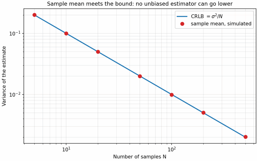
$$\mathrm{var}(\hat{A}) \ge \frac{\sigma^2}{N}$$
The sample mean $\bar{x}$ is unbiased and has variance exactly $\sigma^2/N$. It reaches the bound, so it is efficient and therefore the MVUE for this problem.
Example 2: the amplitude of a known sinusoid
Now measure the amplitude $A$ of a sinusoid with a known frequency $f_0$ and phase $\varphi$, in the same kind of noise:
$$x[n] = A\cos(2\pi f_0 n + \varphi) + w[n]$$
Write $c[n] = \cos(2\pi f_0 n + \varphi)$. The score is $\frac{1}{\sigma^2}\sum_n c[n]\,(x[n] – A\,c[n])$, and the Fisher information is $I(A) = \frac{1}{\sigma^2}\sum_n c[n]^2$. The bound is
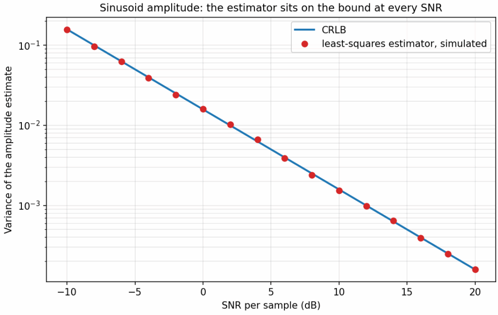
$$\mathrm{var}(\hat{A}) \ge \frac{\sigma^2}{\sum_n c[n]^2} \approx \frac{2\sigma^2}{N}$$
The approximation holds when $f_0$ is not close to 0 or 0.5, because the average of $\cos^2$ is one half. The least-squares estimator
$$\hat{A} = \frac{\sum_n x[n]\,c[n]}{\sum_n c[n]^2}$$
is unbiased and has variance exactly equal to the bound. It is efficient for this problem too.
Python: simulating the bound
The code below runs both examples with 20,000 random datasets each. It compares the simulated variance of each estimator with the CRLB.
import numpy as np

rng = np.random.default_rng(1)

def dc_level_experiment(A=2.0, sigma=1.0, N=50, trials=20_000):
    """Estimate a constant A from N noisy samples with the sample mean."""
    x = A + sigma * rng.standard_normal((trials, N))
    A_hat = x.mean(axis=1)                 # sample mean estimator
    crlb = sigma ** 2 / N                  # CRLB = 1 / Fisher information
    return A_hat.mean(), A_hat.var(), crlb

print("Example 1: DC level in white Gaussian noise")
for N in [10, 50, 200]:
    mean_hat, var_sim, crlb = dc_level_experiment(N=N)
    print(f"  N={N:4d}: mean {mean_hat:.3f}, variance {var_sim:.5f}, CRLB {crlb:.5f}")

def sinusoid_experiment(A=1.0, f0=0.1, phi=0.3, sigma=1.0, N=64, trials=20_000):
    """Estimate the amplitude A of a known sinusoid (known f0 and phase)."""
    n = np.arange(N)
    c = np.cos(2 * np.pi * f0 * n + phi)   # known signal shape, dmu/dA
    x = A * c + sigma * rng.standard_normal((trials, N))
    A_hat = (x @ c) / (c @ c)              # least-squares estimator
    crlb = sigma ** 2 / (c @ c)            # Fisher information = (c @ c) / sigma^2
    return A_hat.mean(), A_hat.var(), crlb

print("Example 2: amplitude of a known sinusoid")
mean_hat, var_sim, crlb = sinusoid_experiment()
print(f"  mean {mean_hat:.4f}, variance {var_sim:.6f}, CRLB {crlb:.6f}")
print(f" ratio variance / CRLB: {var_sim / crlb:.3f}")Running it prints:
Example 1: DC level in white Gaussian noise
  N=  10: mean 1.998, variance 0.09800, CRLB 0.10000
  N=  50: mean 2.000, variance 0.02010, CRLB 0.02000
  N= 200: mean 2.001, variance 0.00496, CRLB 0.00500
Example 2: amplitude of a known sinusoid
  mean 1.0005, variance 0.030986, CRLB 0.031642
ratio variance / CRLB: 0.979The means are close to the true values, so both estimators are unbiased. The simulated variances match the bound to within about 2%, which is the size of the random error in 20,000 trials.
Three common misunderstandings
- “The CRLB is the variance of my estimator.” No. It is a lower limit that holds for every unbiased estimator. Your estimator’s variance is at or above it.
- “If my estimator misses the bound, it is bad.” Not necessarily. The bound may not be reachable for that problem. Compare with the best known estimator before concluding anything.
- “The bound only applies to unbiased estimators, so biased ones are always worse.” Biased estimators are outside the bound’s scope, and they can have smaller variance. Their total error is judged by the mean square error (MSE), which adds the squared bias to the variance. See the MSE post.
Where the bound is used
The CRLB is a planning tool. Before building an estimator, you compute the bound from the signal model and the noise level. If the required accuracy is below the bound, no unbiased estimator can meet it, and the system needs more samples or more power. Once an estimator is built, its simulated variance is compared with the bound to check how close it comes. The phase estimation post applies the same steps to a carrier phase problem.
What comes next
The bound for one parameter is the starting point. The Fisher information and score post explains the quantities in more detail, the MVUE post covers the optimal estimator in general, and the efficient estimators post shows when the bound is reached.
Summary
- An unbiased estimator has an average equal to the true value. Its variance measures how much it scatters.
- The Fisher information measures how sharply the data reveal the parameter.
- The Cramér-Rao bound says no unbiased estimator can have variance below $1/I(\theta)$.
- A sample mean reaches the bound for a constant in Gaussian noise. A least-squares estimator reaches it for a sinusoid’s amplitude.
Learning path: Estimation theory
- Estimation theory introduction
- The mean square error
- Minimum-variance unbiased estimators
- Cramér-Rao lower bound introduction (this post)
- Fisher information and score
- Efficient estimators and the CRLB
- Cramér-Rao bound for phase estimation
References
- Steven M. Kay, Fundamentals of Statistical Signal Processing, Volume I: Estimation Theory, Prentice Hall, 1993. Catalog record. A standard textbook on the Cramér-Rao bound and efficient estimators.
- Cramér-Rao bound (Wikipedia): the general statement and proof outline.
- Fisher information (Wikipedia): the definition and properties.
- Score (statistics) (Wikipedia): the derivative of the log-likelihood.
- Minimum-variance unbiased estimator (Wikipedia): the optimal unbiased estimator.
- Efficiency (statistics) (Wikipedia): what it means for an estimator to reach the bound.
- Harald Cramér (Wikipedia) and C. R. Rao (Wikipedia): the two researchers the bound is named after.
Estimation and detection in communications. The same likelihood and variance tools drive channel estimation, timing recovery and detection in digital receivers. The GaussianWaves eBooks cover that classical side with runnable Python and Matlab code.
Hi, how can I see the latex lines properly? I have tried different browsers (IE, Chrome and Safari) with no luck. What I see is for example “$latex {{sigma}^2}_{hat{theta}} left( theta right ) geq CRLB left( theta right) Rightarrow {sigma}_{hat{theta}} left( theta right ) geq sqrt{CRLB left( theta right)} &s=2$”. Thanks!
Fixed the issue. Please reload the page. Thanks for informing.