Plot FFT using Matlab – FFT of sine wave & cosine wave

Key focus: Learn how to plot FFT of sine wave and cosine wave using Matlab. Understand FFTshift. Plot one-sided, double-sided and normalized spectrum.

Introduction

Numerous texts are available to explain the basics of Discrete Fourier Transform and its very efficient implementation – Fast Fourier Transform (FFT).  Often we are confronted with the need to generate simple, standard signals (sine, cosine, Gaussian pulse, squarewave, isolated rectangular pulse, exponential decay, chirp signal) for simulation purpose. I intend to show (in a series of articles) how these basic signals can be generated in Matlab and how to represent them in frequency domain using FFT. If you are inclined towards Python programming, visit here.

[table id=37/]

Sine Wave

In order to generate a sine wave in Matlab, the first step is to fix the frequency $latex f$ of the sine wave. For example, I intend to generate a f=10 Hz sine wave whose minimum and maximum amplitudes are $latex -1V$ and $latex +1V$ respectively. Now that you have determined the frequency of the sinewave, the next step is to determine the sampling rate. Matlab is a software that processes everything in digital. In order to generate/plot a smooth sine wave, the sampling rate must be far higher than the prescribed minimum required sampling rate which is at least twice the frequency $latex f$ – as per Nyquist Shannon Theorem. A oversampling factor of $latex 30$ is chosen here – this is to plot a smooth continuous-like sine wave (If this is not the requirement, reduce the oversampling factor to desired level). Thus the sampling rate becomes $latex f_s=30 \times f=300 Hz$. If a phase shift is desired for the sine wave, specify it too.

f=10; %frequency of sine wave
overSampRate=30; %oversampling rate
fs=overSampRate*f; %sampling frequency
phase = 1/3*pi; %desired phase shift in radians
nCyl = 5; %to generate five cycles of sine wave

t=0:1/fs:nCyl*1/f; %time base

x=sin(2*pi*f*t+phase); %replace with cos if a cosine wave is desired
plot(t,x);
title(['Sine Wave f=', num2str(f), 'Hz']);
xlabel('Time(s)');
ylabel('Amplitude');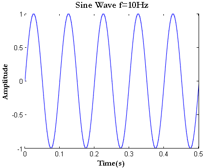

Representing in Frequency Domain

Representing the given signal in frequency domain is done via Fast Fourier Transform (FFT) which implements Discrete Fourier Transform (DFT) in an efficient manner. Usually, power spectrum is desired for analysis in frequency domain. In a power spectrum, power of each frequency component of the given signal is plotted against their respective frequency. The command $latex FFT(x,N)$ computes the $latex N$-point DFT. The number of points – $latex N$ –  in the DFT computation is taken as power of (2) for facilitating efficient computation with FFT. A value of $latex N=1024$ is chosen here. It can also be chosen as next power of 2 of the length of the signal.

Different representations of FFT:

Since FFT is just a numeric computation of $latex N$-point DFT, there are many ways to plot the result.

1. Plotting raw values of DFT:

The x-axis runs from $latex 0$ to $latex N-1$ – representing $latex N$ sample values. Since the DFT values are complex, the magnitude of the DFT $latex abs(X)$ is plotted on the y-axis. From this plot we cannot identify the frequency of the sinusoid that was generated.

NFFT=1024; %NFFT-point DFT      
X=fft(x,NFFT); %compute DFT using FFT        
nVals=0:NFFT-1; %DFT Sample points       
plot(nVals,abs(X));      
title('Double Sided FFT - without FFTShift');        
xlabel('Sample points (N-point DFT)')        
ylabel('DFT Values');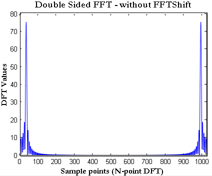

2. FFT plot – plotting raw values against Normalized Frequency axis:

In the next version of plot, the frequency axis (x-axis) is normalized to unity. Just divide the sample index on the x-axis by the length $latex N$ of the FFT. This normalizes the x-axis with respect to the sampling rate $latex f_s$. Still, we cannot figure out the frequency of the sinusoid from the plot.

NFFT=1024; %NFFT-point DFT      
X=fft(x,NFFT); %compute DFT using FFT        
nVals=(0:NFFT-1)/NFFT; %Normalized DFT Sample points         
plot(nVals,abs(X));      
title('Double Sided FFT - without FFTShift');        
xlabel('Normalized Frequency')       
ylabel('DFT Values');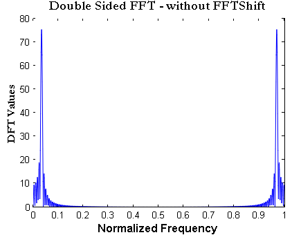

3. FFT plot – plotting raw values against normalized frequency (positive & negative frequencies):

As you know, in the frequency domain, the values take up both positive and negative frequency axis. In order to plot the DFT values on a frequency axis with both positive and negative values, the DFT value at sample index $latex 0$ has to be centered at the middle of the array. This is done by using $latex FFTshift$ function in Matlab. The x-axis runs from $latex -0.5$ to $latex 0.5$ where the end points are the normalized ‘folding frequencies’ with respect to the sampling rate $latex f_s$.

NFFT=1024; %NFFT-point DFT      
X=fftshift(fft(x,NFFT)); %compute DFT using FFT      
fVals=(-NFFT/2:NFFT/2-1)/NFFT; %DFT Sample points        
plot(fVals,abs(X));      
title('Double Sided FFT - with FFTShift');       
xlabel('Normalized Frequency')       
ylabel('DFT Values');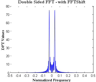

4. FFT plot – Absolute frequency on the x-axis Vs Magnitude on Y-axis:

Here, the normalized frequency axis is just multiplied by the sampling rate. From the plot below we can ascertain that the absolute value of FFT peaks at $latex 10Hz$ and $latex -10Hz$ . Thus the frequency of the generated sinusoid is $latex 10 Hz$. The small side-lobes next to the peak values at $latex 10Hz$ and $latex -10Hz$ are due to spectral leakage.

NFFT=1024;      
X=fftshift(fft(x,NFFT));         
fVals=fs*(-NFFT/2:NFFT/2-1)/NFFT;        
plot(fVals,abs(X),'b');      
title('Double Sided FFT - with FFTShift');       
xlabel('Frequency (Hz)')         
ylabel('|DFT Values|');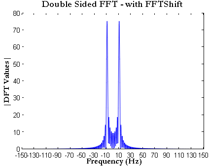

5. Power Spectrum – Absolute frequency on the x-axis Vs Power on Y-axis:

The following is the most important representation of FFT. It plots the power of each frequency component on the y-axis and the frequency on the x-axis. The power can be plotted in linear scale or in log scale. The power of each frequency component is calculated as
$latex P_x(f)=X(f)X^{*}(f)$
Where $latex X(f)$ is the frequency domain representation of the signal $latex x(t)$. In Matlab, the power has to be calculated with proper scaling terms (since the length of the signal and transform length of FFT may differ from case to case).

NFFT=1024;
L=length(x);         
X=fftshift(fft(x,NFFT));         
Px=X.*conj(X)/(NFFT*L); %Power of each freq components       
fVals=fs*(-NFFT/2:NFFT/2-1)/NFFT;        
plot(fVals,Px,'b');      
title('Power Spectral Density');         
xlabel('Frequency (Hz)')         
ylabel('Power');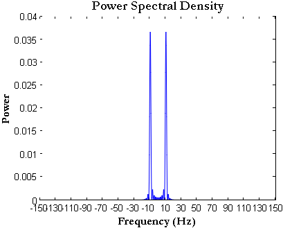

If you wish to verify the total power of the signal from time domain and frequency domain plots, follow this link.
Plotting the power spectral density (PSD) plot with y-axis on log scale, produces the most encountered type of PSD plot in signal processing.

NFFT=1024;      
L=length(x);         
X=fftshift(fft(x,NFFT));         
Px=X.*conj(X)/(NFFT*L); %Power of each freq components       
fVals=fs*(-NFFT/2:NFFT/2-1)/NFFT;        
plot(fVals,10*log10(Px),'b');        
title('Power Spectral Density');         
xlabel('Frequency (Hz)')         
ylabel('Power');

6. Power Spectrum – One-Sided frequencies

In this type of plot, the negative frequency part of x-axis is omitted. Only the FFT values corresponding to $latex 0$ to $latex N/2$ sample points of $latex N$-point DFT are plotted. Correspondingly, the normalized frequency axis runs between $latex 0$ to $latex 0.5$. The absolute frequency (x-axis) runs from $latex 0$ to $latex f_s/2$.

L=length(x);        
NFFT=1024;       
X=fft(x,NFFT);       
Px=X.*conj(X)/(NFFT*L); %Power of each freq components       
fVals=fs*(0:NFFT/2-1)/NFFT;      
plot(fVals,Px(1:NFFT/2),'b','LineSmoothing','on','LineWidth',1);         
title('One Sided Power Spectral Density');       
xlabel('Frequency (Hz)')         
ylabel('PSD');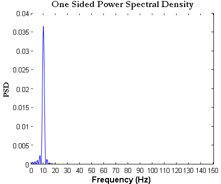

Rate this article: [ratings]

For further reading

[1] Power spectral density – MIT opencourse ware↗

Topics in this chapter

[table id=31 /]

Books by the author

[table id=23 /]