MIMO System Capacity: Unlocking Blazing-Fast Wireless Speeds

Introduction

Extend the scalar ergodic average to a matrix channel. With receiver CSI and equal power across transmit antennas, ergodic MIMO capacity is the expectation of a log-determinant—the expression Telatar and Foschini derived.

Motive

Why bother? Because this one expression predicts the headline gains of MIMO: at high SNR, capacity grows roughly as \(\min(N_t,N_r)\log\rho\). If your simulation does not show that slope from \(1\times 1\) to \(2\times 2\) to \(4\times 4\), something in the normalisation is wrong—and the standards discussion will not make sense until you fix it.

Technical development

For a fixed channel realisation with receiver CSI and total power constraint split equally,

\[C(\mathbf{H})=\log_2\det\!\left(\mathbf{I}_{N_r}+\frac{\rho}{N_t}\mathbf{H}\mathbf{H}^H\right).\]

Ergodic capacity is \(E[C(\mathbf{H})]\). If the transmitter also knows \(\mathbf{H}\), waterfilling over singular values can improve the number; equal power is already near-optimal at high SNR for i.i.d. Rayleigh channels.

How this achieves the motive

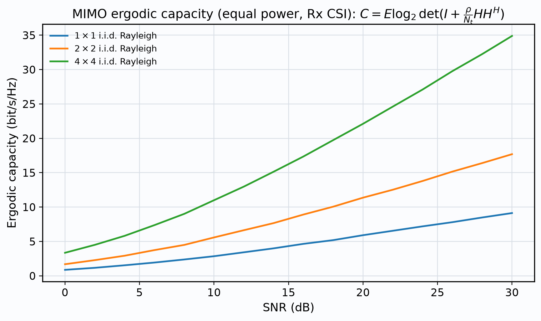
Read the slopes in Figure 1 between 15 and 30 dB. The \(4\times 4\) curve rises about four times as fast as the SISO curve in the \(\log\rho\) sense—visual confirmation of the multiplexing gain \(\min(N_t,N_r)\). At low SNR the curves bunch together: degrees of freedom matter less when every stream is noise-limited.

Sample simulation

import numpy as np
import matplotlib.pyplot as plt

def ergodic_mimo(nt, nr, snr_db, trials=1500, rng=None):
    rng = rng or np.random.default_rng()
    snr = 10 ** (snr_db / 10)
    caps = []
    for _ in range(trials):
        H = (rng.standard_normal((nr, nt)) + 1j * rng.standard_normal((nr, nt))) / np.sqrt(2)
        gram = H @ H.conj().T
        caps.append(np.real(np.linalg.slogdet(np.eye(nr) + (snr / nt) * gram)[1]) / np.log(2))
    return np.mean(caps)

snr_db = np.arange(0, 31, 2)
plt.figure(figsize=(8, 4.5))
for nt, nr in ((1, 1), (2, 2), (4, 4)):
    vals = [ergodic_mimo(nt, nr, s) for s in snr_db]
    plt.plot(snr_db, vals, label="%dx%d" % (nt, nr))
plt.xlabel("SNR (dB)"); plt.ylabel("Ergodic capacity (bit/s/Hz)")
plt.grid(True); plt.legend(); plt.show()

Sample results

Figure 1 is exactly this listing. Increase \(trials\) if the curves look noisy. Compare a point at 20 dB against the Shannon calculator for the scalar AWGN baseline: MIMO should sit well above it when \(\min(N_t,N_r)>1\).

Next topic

Capacity tells you what the channel can carry. The diversity path tells you how to spend antennas on reliability instead. To reconnect the two views, return to the multiple-antenna introduction, or to diversity versus multiplexing.

References

1. I. E. Telatar, “Capacity of multi-antenna Gaussian channels,” European Transactions on Telecommunications, vol. 10, no. 6, pp. 585–595, Nov./Dec. 1999.
2. G. J. Foschini and M. J. Gans, “On limits of wireless communications in a fading environment when using multiple antennas,” Wireless Personal Communications, vol. 6, no. 3, pp. 311–335, Mar. 1998.
3. D. Tse and P. Viswanath, Fundamentals of Wireless Communication, Cambridge University Press, Cambridge, UK, 2005. Chapters 7–8.
4. A. Paulraj, R. Nabar, and D. Gore, Introduction to Space-Time Wireless Communications, Cambridge University Press, Cambridge, UK, 2003.

Frequently asked questions

What is the equal-power MIMO capacity formula with receiver CSI? For a fixed channel, \(C(\mathbf{H})=\log_2\det\bigl(\mathbf{I}_{N_r}+(\rho/N_t)\mathbf{H}\mathbf{H}^H\bigr)\). Ergodic capacity is the expectation of that quantity over the distribution of \(\mathbf{H}\). Equal power across transmit antennas is near-optimal at high SNR for i.i.d. Rayleigh channels.

Why does capacity slope grow with \(\min(N_t,N_r)\) at high SNR? That pre-log factor is the multiplexing gain: the number of parallel spatial streams the channel can support when noise is weak. A square \(4\times 4\) array therefore rises about four times as steeply as SISO on a capacity-versus-\(\log\rho\) plot.

Does waterfilling change the high-SNR slope? With transmitter CSI, waterfilling over singular values improves the constant term and helps at low to moderate SNR, but the high-SNR multiplexing gain remains \(\min(N_t,N_r)\) for full-rank i.i.d. channels.

Who derived the multi-antenna Gaussian capacity results? Telatar’s 1999 European Transactions paper and Foschini and Gans’s 1998 Wireless Personal Communications paper established the information-theoretic foundations that later textbooks and standards build on.