Diversity vs spatial multiplexing — SNR gain or more streams?

Introduction

In one sentence: Diversity spends antennas on reliability (fade averaging); spatial multiplexing spends them on parallel streams — you rarely maximize both at once.

Engineering use: Use this as the map into selection combining, MRC, and MIMO articles; pick the antenna budget that matches your outage vs rate goal.

Motive

Suppose you are designing a Wi-Fi link indoors. With four antennas you might (a) send one stream with heavy space-time coding so the packet survives a fade, or (b) send four streams and hope the channel matrix is well conditioned. Choice (a) lowers error rate; choice (b) raises peak throughput. Before opening a standards document, it helps to have a quantitative feel for that trade.

Technical development

Diversity order

At high SNR, many uncoded or lightly coded error probabilities over Rayleigh fading behave as

\[P_e \asymp G_c \,\mathrm{SNR}^{-d},\]

where \(d\) is the diversity order (the slope on a log–log BER plot) and \(G_c\) is a coding gain that shifts the curve. For an i.i.d. Rayleigh MIMO link the maximum diversity order is \(N_t N_r\). Receive MRC with \(N\) antennas achieves \(d=N\). Selection combining achieves the same order but a worse coding gain—we will see that numerically later.

Multiplexing gain

Ergodic capacity of an i.i.d. MIMO channel with receiver CSI grows, at high SNR, like

\[C(\rho)\approx r\log_2\rho + O(1), \qquad r=\min(N_t,N_r).\]

The pre-log factor \(r\) is the multiplexing gain: how many spatial streams the channel can support in the high-SNR limit. Zheng and Tse showed that a scheme cannot simultaneously achieve the maximum diversity order and the maximum multiplexing gain; there is a trade-off curve \(d(r)\) between them.

How this achieves the motive

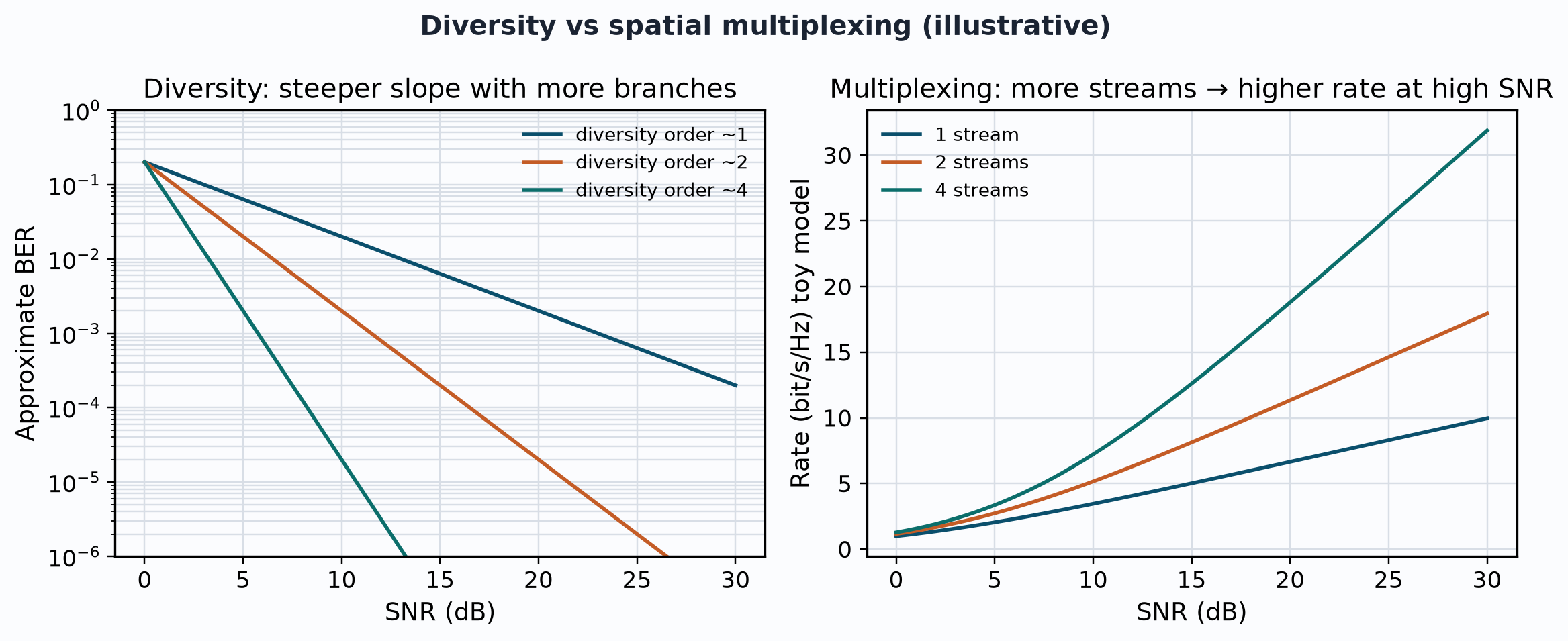
Look at the left panel of Figure 1. Doubling the diversity order does not merely shift the curve; it steepens it. That is why a second receive antenna helps so much at high SNR: outage and BER fall as a higher negative power of SNR. The right panel shows the other choice: more streams raise the degrees of freedom, so capacity grows faster with SNR once each stream is above noise.

In practice a link rarely sits at either extreme. LTE and NR pick a number of layers from channel-state feedback, use codebook precoding that mixes beamforming and multiplexing, and still rely on coding across time and frequency for diversity. The pictures above are a good place to start when reading those choices.

Sample simulation

The listing below draws the two panels of Figure 1. The BER curves are not a full link simulation; they use the high-SNR form \(P_e\propto\mathrm{SNR}^{-N}\) so the slopes are visible without a Monte Carlo run. The rate curves split total power equally across \(k\) parallel AWGN channels—a simple model of spatial multiplexing.

import numpy as np
import matplotlib.pyplot as plt

snr_db = np.linspace(0, 30, 61)
snr = 10 ** (snr_db / 10)

plt.figure(figsize=(10, 4))
plt.subplot(1, 2, 1)
for N in (1, 2, 4):
    plt.semilogy(snr_db, 0.2 / snr ** N, label="diversity order ~%d" % N)
plt.xlabel("SNR (dB)"); plt.ylabel("Approximate BER"); plt.grid(True); plt.legend()

plt.subplot(1, 2, 2)
for k in (1, 2, 4):
    plt.plot(snr_db, k * np.log2(1 + snr / k), label="%d streams" % k)
plt.xlabel("SNR (dB)"); plt.ylabel("Rate (bit/s/Hz)"); plt.grid(True); plt.legend()
plt.tight_layout(); plt.show()

Sample results

On the BER panel, compare the gap between \(N=1\) and \(N=2\) at \(10^{-4}\): it is tens of decibels for this asymptotic model, which is the point of receive diversity even though the prefactor \(0.2\) is arbitrary. On the rate panel, four streams pull ahead at high SNR but the advantage shrinks at low SNR—the regime where a single robust stream is often preferred.

Next topic

Next we treat receive diversity on its own: one transmit antenna and several receive antennas. The following article writes the SIMO model and introduces the linear combiners—selection, MRC, and equal gain—that turn those antennas into a single decision statistic.

References

1. D. Tse and P. Viswanath, Fundamentals of Wireless Communication, Cambridge University Press, Cambridge, UK, 2005. Chapters 3 and 9.
2. L. Zheng and D. N. C. Tse, “Diversity and multiplexing: A fundamental tradeoff,” IEEE Transactions on Information Theory, vol. 49, no. 5, pp. 1073–1096, May 2003.
3. A. Goldsmith, Wireless Communications, Cambridge University Press, Cambridge, UK, 2005.

Frequently asked questions

Can spatial diversity and spatial multiplexing be maximised at the same time? Not at every operating point. Zheng and Tse showed a fundamental trade-off: schemes that push multiplexing gain toward \(\min(N_t,N_r)\) must give up diversity order, and schemes that aim for full diversity order \(N_t N_r\) must reduce the number of independent streams. Practical links choose an intermediate point from channel quality feedback.

What is diversity order on a bit-error-rate plot? At high SNR, many error probabilities over Rayleigh fading behave as \(P_e \propto \mathrm{SNR}^{-d}\). The exponent \(d\) is the diversity order—the slope on a log–log BER plot. Receive MRC with \(N\) independent branches achieves \(d=N\).

What is multiplexing gain in capacity formulas? Ergodic MIMO capacity with receiver CSI grows approximately as \(r\log_2\rho\) at high SNR, where \(r=\min(N_t,N_r)\). The pre-log factor \(r\) is the multiplexing gain: how many spatial streams the channel can support when noise is no longer the limiting factor.

How do LTE and 5G NR choose between diversity and multiplexing? The scheduler and outer loop pick a number of layers (rank) from CSI reports. Poor channel quality or a nearly rank-one matrix favours transmit diversity or a single beamformed stream; a well-conditioned channel at high SNR favours more layers. Coding across time and frequency still supplies diversity even when several streams are active.