Simulation of Rayleigh Fading ( Clarke’s Model – sum of sinusoids method)

Note: There is a rating embedded within this post, please visit this post to rate it.

A multipath fading channel  can be modeled as a FIR (Finite Impulse Response) filter with the following impulse response.

$$ h( \tau ; t ) = h_{0}(t) \delta ( \tau – \tau_{0}(t)) + h_{1}(t) \delta ( \tau – \tau_{1}(t)) + . . . + h_{L-1}(t) \delta ( \tau – \tau_{L-1}(t)) $$

where h(τ,t) is the time varying impulse response of the multipath fading channel having L multipaths and hi(t) and τi(t) denote the time varying complex gain and excess delay of the i-th path. The above mentioned impulse response can be implemented as a FIR filter as shown below :

Multipath Fading phenomena – modelled as a Time Varying FIR Filter

The channel under consideration can be modeled as a multipath fading channel in which the impulse response may follow distributions like Rayleigh distribution ( in which there is no Line of Sight (LOS) ray between transmitter and receiver) or as Rician distribution ( dominant LOS path exist between transmitter and receiver), Nagami distribution, Weibull distribution etc.

Different methods of simulation techniques were proposed to simulate/model multipath channels. Some of the models include clarke’s reference model, Jake’s model, Young’s model , filtered gaussian noise model etc.

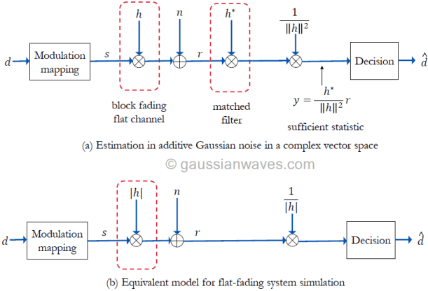
A Rayleigh fading channel (flat fading channel) is considered in this text.For simplicity we fix the excess delays τi(t) in the above equation and we generate hi(t) that follows Rayleigh distribution. In this simulation Clarke’s Rayleigh fading model is used. This model is also called mathematical reference model and is commonly considered as a computationally inefficient model compared to Jake’s Rayleigh Fading simulator.

Theory of Rayleigh Fading:

Lets denote the complex impulse response h(t) of the flat fading channel as follows :

$$ h(t) = h_{I}(t) + jh_{Q}(t) $$

where hI(t) and hQ(t) are zero mean gaussian distributed. Therefore the fading envelope is Rayleigh distributed and is given by

$$ \left |h(t) \right | = \sqrt{\left |h_{I}(t) \right |^2 + \left |h_{Q}(t) \right |^2} $$

The probability density function (Rayleigh distribution) of the above mentioned amplitude response is given by

$$ f(z)=\frac{2z}{\sigma ^{2}}e^{-\frac{z^{2}}{\sigma ^{2}}} \\ where \; \sigma ^{2} = E\left ( \left | h(t) \right |^{2} \right ) $$

We will use the Clarke’s Rayleigh Fading model (given below) and check the statistical properties of the random process generated by the model against the statistical properties of Rayleigh distribution (given above).

Clarke’s Rayleigh Fading model:

The random process of flat Rayleigh fading with M multipaths can be simulated with the sum-of-sinusoid method described as

Simulation:

1) The rayleigh fading model is implemented as a function in matlab with following parameters:
M=number of multipaths in the fading channel, N = number of samples to generate, fd=maximum Doppler spread in Hz, Ts = sampling period.

function [h]=rayleighFading(M,N,fd,Ts)

% function to generate rayleigh Fading samples based on Clarke's model
% M = number of multipaths in the channel
% N = number of samples to generate
% fd = maximum Doppler frequency
% Ts = sampling period
% Author : Mathuranathan for https://www.gaussianwaves.com
%Code available in the ebook - Simulation of Digital Communication Systems using Matlab

Check this book for full Matlab code.
Simulation of Digital Communication Systems Using Matlab – by Mathuranathan Viswanathan

2)The above mentioned function is used to generate Rayleigh Fading samples with the following values for the function arguments. M=15; N=10^5; fd=100 Hz;Ts=0.0001 second;

Investigation of Statistical Properties of samples generated using Clarke’s model:

3) Mean and Variance of the real and imaginary parts of generated samples are
Mean of real part ~=0
Mean of imag part ~=0
Variance of real part = 0.4989 ~=0.5
Variance of imag part = 0.4989 ~=0.5

The results implies that the mean of the real and imaginary parts are same and are equal to zero.The variance of the real and imaginary parts are approximately equal to 0.5.

4)Next, the pdf of the real part of the simulated samples are plotted and compared against the pdf of Gaussian distribution (with mean=0 and variance =0.5)

Real Part of simulated samples exhibiting Gaussian Distribution characteristics

5)The pdf of the generated Rayleigh fading samples are plotted and compared against pdf of Rayleigh distribution (with variance=1)

PDF of simulated Rayleigh Fading Samples

6) From 4) and 5) we confirm that the samples generated by Clarke’s model follows Rayleigh distribution (with variance = 1) and the real and imaginary part of the samples follow Gaussian distribution (with mean=0 and variance =0.5).

7) The Magnitude and Phase response of the generated Rayleigh Fading samples are plotted here.

The Magnitude and Phase response of the generated Rayleigh Fading samples

See also

[1]Eb/N0 Vs BER for BPSK over Rayleigh Channel and AWGN Channel
[2]Eb/N0 Vs BER for BPSK over Rician Fading Channel
[3]Performance comparison of Digital Modulation techniques
[4]BER Vs Eb/N0 for BPSK modulation over AWGN
[5]Rayleigh Fading Simulation – Young’s model
[6]Introduction to Fading Channels
[7] Chi-Squared distribution

Recommended Books

External Resources

[1]Theoretical expressions for BER under various conditions

Correlative Coding – Modified Duobinary Signaling

Modified Duobinary Signaling is an extension of duobinary signaling. It has the advantage of zero PSD at low frequencies (especially at DC ) that is suitable for channels with poor DC response. It correlates two symbols that are 2T time instants apart, whereas in duobinary signaling, symbols that are 1T apart are correlated.

The general condition to achieve zero ISI is given by

As discussed in a previous article, in correlative coding , the requirement of zero ISI condition is relaxed as a controlled amount of ISI is introduced in the transmitted signal and is counteracted in the receiver side

In the case of modified duobinary signaling, the above equation is modified as

which states that the ISI is limited to two alternate samples. Here a controlled or “deterministic” amount of ISI is introduced and hence its effect can be removed upon signal detection at the receiver.

Modified Duobinary Signaling:

The following figure shows the modified duobinary signaling scheme (click to enlarge).

Modified DuoBinary Signaling

Encoding Process:

1) an = binary input bit; an ∈ {0,1}.
2) bn = NRZ polar output of Level converter in the precoder and is given by,

where ak is the precoded output (before level converter).

3) yn can be represented as

Note that the samples bn are uncorrelated ( i.e either +d for “1” or -d for “0” input). On the other-hand,the samples yn are correlated ( i.e. there are three possible values +2d,0,-2d depending on ak and ak-2). Meaning that the modified duobinary encoding correlates present sample ak and the previous input sample ak-2.

4) From the diagram,impulse response of the modified duobinary encoder is computed as

Decoding Process:

5) The receiver consists of a modified duobinary decoder and a postcoder (inverse of precoder). The decoder implements the following equation (which can be deduced from the equation given under step 3 (see above))

This equation indicates that the decoding process is prone to error propagation as the estimate of present sample relies on the estimate of previous sample. This error propagation is avoided by using a precoder before modified-duobinary encoder at the transmitter and a postcoder after the modified-duobinary decoder. The precoder ties the present sample and the sample that precedes the previous sample ( correlates these two samples) and the postcoder does the reverse process.

6) The entire process of modified-duobinary decoding and the postcoding can be combined together as one algorithm. The following decision rule is used for detecting the original modified-duobinary signal samples {an} from {yn}

Matlab code:

Check this book for full Matlab code.
Wireless Communication Systems in Matlab – by Mathuranathan Viswanathan

Simulation Results:

To know more on the simulation and results – visit this page – “Partial response signalling schemes – impulse and frequency responses”

Impulse response and frequency response of various Partial response (PR) signaling schemes

Rate this post: Note: There is a rating embedded within this post, please visit this post to rate it.

See also :

[1] Correlative Coding – Duobinary Signaling
[2] Introduction to Inter Symbol Interference

Recommended Books

Correlative coding – Duobinary Signaling

The condition for zero ISI (Inter Symbol Interference) is

which states that when sampling a particular symbol (at time instant nT=0), the effect of all other symbols on the current sampled symbol is zero.

As discussed in the previous article, one of the practical ways to mitigate ISI is to use partial response signaling technique ( otherwise called as “correlative coding”). In partial response signaling, the requirement of zero ISI condition is relaxed as a controlled amount of ISI is introduced in the transmitted signal and is counteracted in the receiver side.

By relaxing the zero ISI condition, the above equation can be modified as,

which states that the ISI is limited to two adjacent samples. Here we introduce a controlled or “deterministic” amount of ISI and hence its effect can be removed upon signal detection at the receiver.

Duobinary Signaling:

The following figure shows the duobinary signaling scheme.

Figure 1: DuoBinary signaling scheme

Encoding Process:

1) an = binary input bit; an ∈ {0,1}.
2) bn = NRZ polar output of Level converter in the precoder and is given by,

3) yn can be represented as

Note that the samples bn are uncorrelated ( i.e either +d for “1” or -d for “0” input). On the other-hand, the samples yn are correlated ( i.e. there are three possible values +2d,0,-2d depending on an and an-1). Meaning that the duobinary encoding correlates present sample an and the previous input sample an-1.

4) From the diagram,impulse response of the duobinary encoder is computed as

Decoding Process:

5) The receiver consists of a duobinary decoder and a postcoder (inverse of precoder).The duobinary decoder implements the following equation (which can be deduced from the equation given under step 3 (see above))

This equation indicates that the decoding process is prone to error propagation as the estimate of present sample relies on the estimate of previous sample. This error propagation is avoided by using a precoder before duobinary encoder at the transmitter and a postcoder after the duobinary decoder. The precoder ties the present sample and previous sample ( correlates these two samples) and the postcoder does the reverse process.

6) The entire process of duobinary decoding and the postcoding can be combined together as one algorithm. The following decision rule is used for detecting the original duobinary signal samples {an} from {yn}

Matlab Code:

Check this book for full Matlab code and simulation results.
Wireless Communication Systems in Matlab – by Mathuranathan Viswanathan

Simulation and results

To know more on the simulation and results – visit this page – “Partial response signalling schemes – impulse and frequency responses”

Impulse response and frequency response of various Partial response (PR) signaling schemes

Rate this article: Note: There is a rating embedded within this post, please visit this post to rate it.

See also :

[1] Correlative Coding – Modified Duobinary Signaling
[2] Derivation of expression for a Gaussian Filter with 3 dB bandwidth
[3] Nyquist and Shannon Theorem
[4] Correlative coding – Duobinary Signaling
[5] Square Root Raised Cosine Filter (Matched/split filter implementation)
[6] Introduction to Inter Symbol Interference

External Resources:

[1] The care and feeding of digital, pulse-shaping filters – By Ken Gentile↗
[2] Inter Symbol Interference and Root Raised Cosine Filtering – Complex2real↗

Young’s model for Rayleigh fading

Introduction

Young’s fading channel model is a mathematical model used to describe the behavior of a wireless communication channel. It is a type of frequency selective fading channel model that is commonly used to simulate the effects of multipath interference on wireless signals.

The model is based on the assumption that the transmitted signal reaches the receiver through multiple paths, each with a different attenuation and phase shift. The attenuation and phase shift of each path are modeled as independent random variables with specific probability distributions.

The model uses the sum of these attenuated and phase-shifted paths to simulate the received signal. The resulting signal experiences fading due to the constructive and destructive interference of the individual paths.

Young’s fading channel model is useful for simulating the performance of wireless communication systems in a multipath environment. It can help researchers and engineers evaluate the performance of different modulation and coding schemes and develop techniques to mitigate the effects of fading.

Young’s model

In the previous article, the characteristics and types of fading was discussed. Rayleigh Fading channel with Doppler shift is considered in this article.

Consider a channel affected by both Rayleigh Fading phenomena and Doppler Shift. Rayleigh Fading is caused due to multipath reflections of the received signal before it reaches the receiver and the Doppler Shift is caused due to the difference in the relative velocity/motion between the transmitter and the receiver. This scenario is encountered in day to day mobile communications.

A number of simulation algorithms are proposed for generation of correlated Rayleigh random variables. David J.Young and Norman C Beaulieu proposed a method in their paper titled “The Generation of Correlated Rayleigh Random Variates by Inverse Discrete Fourier Transform”[1] based on the inverse discrete Fourier transform (IDFT). It is a modification of the Smith’s algorithm which is normally used for Rayleigh fading simulation. This method requires exactly one-half the number of IDFT operations and roughly two-thirds the computer memory of the original method – as the authors of the paper claims.

Rayleigh Fading can be simulated by adding two Gaussian Random variables as mentioned in my previous post. The effect of Doppler shift is incorporated by modeling the Doppler effect as a frequency domain filter.

The model proposed by Young et.al is shown below.

Rayleigh Fading – Young’s model

The Fading effect + Doppler Shift is simulated by multiplying the Gaussian Random variables and the Doppler Shift’s Frequency domain representation. Then IDFT is performed to bring them into time domain representation. The Doppler Filter used to represent the Doppler Shift effect is derived in Young’s paper.

The equation for the Doppler Filter is :

Matlab Code

Check this book for full Matlab code.
Simulation of Digital Communication Systems Using Matlab – by Mathuranathan Viswanathan

Matlab code Output:

Rayleigh Fading with Doppler Effect

Reference:

[1] D.J. Young and N.C. Beaulieu, “The generation of correlated Rayleigh random variates by inverse discrete fourier transform,” IEEE transactions on Communications, vol. 48, pp. 1114-1127, July 2000.

See also

[1]Eb/N0 Vs BER for BPSK over Rayleigh Channel and AWGN Channel
[2]Simulation of Rayleigh Fading ( Clarke’s Model – sum of sinusoids method)
[3]Performance comparison of Digital Modulation techniques
[4]BER Vs Eb/N0 for BPSK modulation over AWGN
[5]Introduction to Fading Channels

External Resources

[1]Theoretical expressions for BER under various conditions
[2]Capacity of MRC on correlated Rician Fading Channels

Fading channel – complex baseband equivalent models

Keyfocus: Fading channel models for simulation. Learn how fading channels can be modeled as FIR filters for simplified modulation & detection. Rayleigh/Rician fading.

Introduction

A fading channel is a wireless communication channel in which the quality of the signal fluctuates over time due to changes in the transmission environment. These changes can be caused by different factors such as distance, obstacles, and interference, resulting in attenuation and phase shifting. The signal fluctuations can cause errors or loss of information during transmission.

Fading channels are categorized into slow fading and fast fading depending on the rate of channel variation. Slow fading occurs over long periods, while fast fading happens rapidly over short periods, typically due to multipath interference.

To overcome the negative effects of fading, various techniques are used, including diversity techniques, equalization, and channel coding.

Fading channel in frequency domain

With respect to the frequency domain characteristics, the fading channels can be classified into frequency selective and frequency-flat fading.

A frequency flat fading channel is a wireless communication channel where the attenuation and phase shift of the signal are constant across the entire frequency band. This means that the signal experiences the same amount of fading at all frequencies, and there is no frequency-dependent distortion of the signal.

In contrast, a frequency selective fading channel is a wireless communication channel where the attenuation and phase shift of the signal vary with frequency. This means that the signal experiences different levels of fading at different frequencies, resulting in a frequency-dependent distortion of the signal.

Frequency selective fading can occur due to various factors such as multipath interference and the presence of objects that scatter or absorb certain frequencies more than others. To mitigate the effects of frequency selective fading, various techniques can be used, such as equalization and frequency hopping.

The channel fading can be modeled with different statistics like Rayleigh, Rician, Nakagami fading. The fading channel models, in this section, are utilized for obtaining the simulated performance of various modulations over Rayleigh flat fading and Rician flat fading channels. Modeling of frequency selective fading channel is discussed in this article.

Linear time invariant channel model and FIR filters

The most significant feature of a real world channel is that the channel does not immediately respond to the input. Physically, this indicates some sort of inertia built into the channel/medium, that takes some time to respond. As a consequence, it may introduce distortion effects like inter-symbol interference (ISI) at the channel output. Such effects are best studied with the linear time invariant (LTI) channel model, given in Figure 1.

Figure 1: Complex baseband equivalent LTI channel model

In this model, the channel response to any input depends only on the channel impulse response(CIR) function of the channel. The CIR is usually defined for finite length \(L\) as \(\mathbf{h}=[h_0,h_1,h_2, \cdots,h_{L-1}]\) where \(h_0\) is the CIR at symbol sampling instant \(0T_{sym}\) and \(h_{L-1}\) is the CIR at symbol sampling instant \((L-1)T_{sym}\). Such a channel can be modeled as a tapped delay line (TDL) filter, otherwise called finite impulse response (FIR) filter. Here, we only consider the CIR at symbol sampling instances. It is well known that the output of such a channel (\(\mathbf{r}\)) is given as the linear convolution of the input symbols (\(\mathbf{s}\)) and the CIR (\(\mathbf{h}\)) at symbol sampling instances. In addition, channel noise in the form of AWGN can also be included the model. Therefore, the resulting vector of from the entire channel model is given as

\[\mathbf{r} = \mathbf{h} \ast \mathbf{s} +\mathbf{n} \quad\quad (1) \]

This article is part of the following books
Digital Modulations using Matlab : Build Simulation Models from Scratch, ISBN: 978-1521493885
Digital Modulations using Python ISBN: 978-1712321638
Wireless communication systems in Matlab ISBN: 979-8648350779
All books available in ebook (PDF) and Paperback formats

Simulation model for detection in flat fading channel

A flat-fading (also called as frequency-non-selective) channel is modeled with a single tap (\(L=1\)) FIR filter with the tap weights drawn from distributions like Rayleigh, Rician or Nakagami distributions. We will assume block fading, which implies that the fading process is approximately constant for a given transmission interval. For block fading, the random tap coefficient \(h=h[0]\) is a complex random variable (not random processes) and for each channel realization, a new set of complex random values are drawn from Rayleigh or Rician or Nakagami fading according to the type of fading desired.

Figure 2: LTI channel viewed as tapped delay line filter

Simulation models for modulation and detection over a fading channel is shown in Figure 2. For a flat fading channel, the output of the channel can be expressed simply as the product of time varying channel response and the input signal. Thus, equation (1) can be simplified (refer this article for derivation) as follows for the flat fading channel.

\[\mathbf{r} = h\mathbf{s} + \mathbf{n} \quad\quad (2) \]

Since the channel and noise are modeled as a complex vectors, the detection of \(\mathbf{s}\) from the received signal is an estimation problem in the complex vector space.

Assuming perfect channel knowledge at the receiver and coherent detection, the receiver shown in Figure 3(a) performs matched filtering. The impulse response of the matched filter is matched to the impulse response of the flat-fading channel as \( h^{\ast}\). The output of the matched filter is scaled down by a factor of \(||h||^2\) which is the total-energy contained in the impulse response of the flat-fading channel. The resulting decision vector \(\mathbf{y}\) serves as the sufficient statistic for the estimation of \(\mathbf{s}\) from the received signal \(\mathbf{r}\) (refer equation A.77 in reference [1])

\[\tilde{\mathbf{y}} = \frac{h^{\ast}}{||h||^2} \mathbf{r} = \frac{h^{\ast}}{||h||^2} h\mathbf{s} + \frac{h^{\ast}}{||h||^2} \mathbf{n} = \mathbf{s} + \tilde{\mathbf{w}} \quad\quad (3) \]

Since the absolute value \(|h|\) and the Eucliden norm \(||h||\) are related as \(|h|^2= \left\lVert h\right\rVert = hh^{\ast}\), the model can be simplified further as given in Figure 3(b).

To simulate flat fading, the values for the fading variable \(h\) are drawn from complex normal distribution

\[h= X + jY \quad\quad (4) \]

where, \(X,Y\) are statistically independent real valued normal random variables.

● If \(E[h]=0\), then \(|h|\) is Rayleigh distributed, resulting in a Rayleigh flat fading channel
● If \(E[h] \neq 0\), then \(|h|\) is Rician distributed, resulting in a Rician flat fading channel with the factor \(K=[E[h]]^2/\sigma^2_h\)

References

[1] D. Tse and P. Viswanath, Fundamentals of Wireless Communication, Cambridge University Press, 2005.↗

Books by the author


Wireless Communication Systems in Matlab
Second Edition(PDF)

(173 votes, average: 3.66 out of 5)

Checkout Added to cart

Digital Modulations using Python
(PDF ebook)

(127 votes, average: 3.58 out of 5)

Checkout Added to cart

Digital Modulations using Matlab
(PDF ebook)

(134 votes, average: 3.63 out of 5)

Checkout Added to cart
Hand-picked Best books on Communication Engineering
Best books on Signal Processing

Hard and Soft decision decoding

What are hard and soft decision decoding

Hard decision decoding and soft decision decoding are two different methods used for decoding error-correcting codes.

With hard decision decoding, the received signal is compared to a set threshold value to determine whether the transmitted bit is a 0 or a 1. This is commonly used in digital communication systems that experience noise or interference, resulting in a low signal-to-noise ratio.

Soft decision decoding, on the other hand, treats the received signal as a probability distribution and calculates the likelihood of each possible transmitted bit based on the characteristics of the received signal. This approach is often used in modern digital communication and data storage systems where the signal-to-noise ratio is relatively high and there is a need for higher accuracy and reliability.

While soft decision decoding can achieve better error correction, it is more complex and computationally expensive than hard decision decoding.

More details

Let’s expatiate on the concepts of hard decision and soft decision decoding. Consider a simple even parity encoder given below.

Input Bit 1
Input Bit 2
Parity bit added by encoder
Codeword Generated
0
0
0
000
0
1
1
011
1
0
1
101
1
1
0
110

The set of all possible codewords generated by the encoder are 000,011,101 and 110.

Lets say we are want to transmit the message “01” through a communication channel.

Hard decision decoding

Case 1 : Assume that our communication model consists of a parity encoder, communication channel (attenuates the data randomly) and a hard decision decoder

The message bits “01” are applied to the parity encoder and we get “011” as the output codeword.

Figure 1: Hard decision decoding – a simple illustration

The output codeword “011” is transmitted through the channel. “0” is transmitted as “0 Volt and “1” as “1 Volt”. The channel attenuates the signal that is being transmitted and the receiver sees a distorted waveform ( “Red color waveform”). The hard decision decoder makes a decision based on the threshold voltage. In our case the threshold voltage is chosen as 0.5 Volt ( midway between “0” and “1” Volt ) . At each sampling instant in the receiver (as shown in the figure above) the hard decision detector determines the state of the bit to be “0” if the voltage level falls below the threshold and “1” if the voltage level is above the threshold. Therefore, the output of the hard decision block is “001”. Perhaps this “001” output is not a valid codeword ( compare this with the all possible codewords given in the table above) , which implies that the message bits cannot be recovered properly. The decoder compares the output of the hard decision block with the all possible codewords and computes the minimum Hamming distance for each case (as illustrated in the table below).

All possible Codewords
Hard decision output
Hamming distance
000
001
1
011
001
1
101
001
1
110
001
3

The decoder’s job is to choose a valid codeword which has the minimum Hamming distance. In our case, the minimum Hamming distance is “1” and there are 3 valid codewords with this distance. The decoder may choose any of the three possibility and the probability of getting the correct codeword (“001” – this is what we transmitted) is always 1/3. So when the hard decision decoding is employed the probability of recovering our data ( in this particular case) is 1/3. Lets see what “Soft decision decoding” offers …

Soft Decision Decoding

The difference between hard and soft decision decoder is as follows

  • In Hard decision decoding, the received codeword is compared with the all possible codewords and the codeword which gives the minimum Hamming distance is selected
  • In Soft decision decoding, the received codeword is compared with the all possible codewords and the codeword which gives the minimum Euclidean distance is selected. Thus the soft decision decoding improves the decision making process by supplying additional reliability information ( calculated Euclidean distance or calculated log-likelihood ratio)

For the same encoder and channel combination lets see the effect of replacing the hard decision block with a soft decision block.

Voltage levels of the received signal at each sampling instant are shown in the figure. The soft decision block calculates the Euclidean distance between the received signal and the all possible codewords.

Valid codewords
Voltage levels at each sampling instant of received waveform
Euclidean distance calculation
Euclidean distance
0 0 0
( 0V 0V 0V )
0.2V 0.4V 0.7V
(0-0.2)2+ (0-0.4)2+ (0-0.7)2
0.69
0 1 1
( 0V 1V 1V )
0.2V 0.4V 0.7V
(0-0.2)2+ (1-0.4)2+ (1-0.7)2
0.49
1 0 1
( 1V 0V 1V )
0.2V 0.4V 0.7V
(1-0.2)2+ (0-0.4)2+ (1-0.7)2
0.89
1 1 0
( 1V 1V 0V )
 
0.2V 0.4V 0.7V
(1-0.2)2+ (1-0.4)2+ (0-0.7)2
1.49

The minimum Euclidean distance is “0.49” corresponding to “0 1 1” codeword (which is what we transmitted). The decoder selects this codeword as the output. Even though the parity encoder cannot correct errors, the soft decision scheme helped in recovering the data in this case. This fact delineates the improvement that will be seen when this soft decision scheme is used in combination with forward error correcting (FEC) schemes like convolution codes , LDPC etc

From this illustration we can understand that the soft decision decoders uses all of the information ( voltage levels in this case) in the process of decision making whereas the hard decision decoders does not fully utilize the information available in the received signal (evident from calculating Hamming distance just by comparing the signal level with the threshold whereby neglecting the actual voltage levels).

Note: This is just to illustrate the concept of Soft decision and Hard decision decoding. Prudent souls will be quick enough to find that the parity code example will fail for other voltage levels (e.g. : 0.2V , 0.4 V and 0.6V) . This is because the parity encoders are not capable of correcting errors but are capable of detecting single bit errors.

Soft decision decoding scheme is often realized using Viterbi decoders. Such decoders utilize Soft Output Viterbi Algorithm (SOVA) which takes into account the apriori probabilities of the input symbols producing a soft output indicating the reliability of the decision.

Rate this article: Note: There is a rating embedded within this post, please visit this post to rate it.

For further reading

[1] I. Dokmanic, R. Parhizkar, J. Ranieri and M. Vetterli, “Euclidean Distance Matrices: Essential theory, algorithms, and applications,” in IEEE Signal Processing Magazine, vol. 32, no. 6, pp. 12-30, Nov. 2015, doi: 10.1109/MSP.2015.2398954.↗

Books by the author


Wireless Communication Systems in Matlab
Second Edition(PDF)

Note: There is a rating embedded within this post, please visit this post to rate it.
Checkout Added to cart

Digital Modulations using Python
(PDF ebook)

Note: There is a rating embedded within this post, please visit this post to rate it.
Checkout Added to cart

Digital Modulations using Matlab
(PDF ebook)

Note: There is a rating embedded within this post, please visit this post to rate it.
Checkout Added to cart
Hand-picked Best books on Communication Engineering
Best books on Signal Processing