Channel Modelling Archives

Euclidean and Hamming distances

Key focus: Euclidean & Hamming distances are used to measure similarity or dissimilarity between two sequences. Used in Soft & Hard decision decoding.

Distance is a measure that indicates either similarity or dissimilarity between two words. Given a pair of words a=(a₀,a₁, … ,a_n-1) and b=(b₀,b₁,…,b_n-1) , there are variety of ways one can characterize the distance, d(a,b), between the two words. Euclidean and Hamming distances are familiar ones. Euclidean distance is extensively applied in analysis of convolutional codes and Trellis codes. Hamming distance is frequently encountered in the analysis of block codes.

This article is part of the book
● Wireless Communication Systems in Matlab (second edition), ISBN: 979-8648350779 available in ebook (PDF) format and Paperback (hardcopy) format.

Euclidean distance

The Euclidean distance between the two words is defined as

\[d_{Euclidean}(\mathbf{a},\mathbf{b}) = \sqrt{(a_0-b_0)^2+(a_1-b_1)^2 + \cdots + (a_{n-1}-b_{n-1})^2}\]

Soft decision decoding

In contrast to classical hard-decision decoders (see below) which operate on binary values, a soft-decision decoder directly processes the unquantized (or quantized in more than two levels in practice) samples at the output of the matched filter for each bit-period, thereby avoiding the loss of information.

If the outputs of the matched filter at each bit-period are unquantized or quantized in more than two levels, the demodulator is said to make soft-decisions. The process of decoding the soft-decision received sequence is called soft-decision decoding. Since the decoder uses the additional information contained in the multi-level quantized or unquantized received sequence, soft-decision decoding provides better performance compared to hard-decision decoding. For soft-decision decoding, metrics like likelihood function, Euclidean distance and correlation are used.

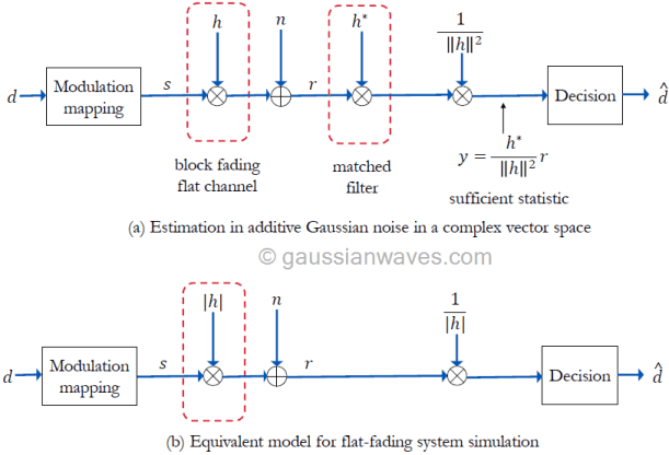
For illustration purposes, we consider the communication system model shown in Figure 1. A block encoder encodes the information blocks m=(m₁,m₂,…,m_k) and generates the corresponding codeword vector c=(c₁,c₂,…,c_n). The codewords are modulated and sent across an AWGN channel. The received signal is passed through a matched filter and the multi-level quantizer outputs the soft-decision vector r .

*Figure 1: Soft-decision receiver model for decoding linear block codes for AWGN channel*

Soft-decision receiver model for decoding linear block codes for AWGN channel (Euclidean Hamming distances) — *Figure 1: Soft-decision receiver model for decoding linear block codes for AWGN channel*

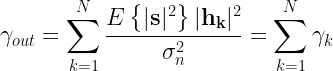
The goal of a decoder is to produce an estimate m̂ of the information sequence m based on the received sequence r. Equivalently, the information sequence m and the codeword c has one-to-one correspondence, the decoder can also produce an estimate ĉ of the codeword c. If the codeword c was transmitted, a decoding error occurs if ĉ ≠ c.

For equi-probable codewords, The decoder that selects a codeword that maximizes the conditional probability P(r, c). This is called a maximum lihelihood decoder (MLD).

For an AWGN channel with two-sided power spectral density N₀/2, the conditional probability is given by

\[P\left(\mathbf{r} | \mathbf{c}\right) = \frac{1}{\left(\pi N_0\right)^{-n/2}} exp \left\lbrace – \sum_{i=1}^{n} \left[r_i – s_i\right]^2 \right\rbrace\]

The sum is the squared Euclidean distance between the received sequence r and the coded signal sequence s. We can note that the term is common for all codewords and n is a constant. This simplifies the MLD decoding rule where we select a codeword from the code dictionary that minimizes the Euclidean distance D(r, s)$.

Hamming distance

Hamming distance between two words a=(a₀,a₁, … ,a_n-1) and b=(b₀,b₁,…,b_n-1) in Galois Field GF(2), is the number of coordinates in which the two blocks differ.

\[d_{Hamming} = d_H(\mathbf{a},\mathbf{b}) = \#\{j : a_j \neq b_j, j = 0,1,\cdots,n-1\}\]

For example, the Hamming distance between (0,0,0,1) and (1,0,1,0) in GF(2) is 3, since they differ in three digits. For an independent and identically distributed (i.i.d) error model with (discrete) uniform error amplitude distribution, the most appropriate measure is Hamming distance.

Minimum distance

The minimum distance of block code C, is the smallest distance between all distance pairs of code words in C. The minimum distance of a block code determines both its error-detecting ability and error-correcting ability. A large minimum distance guarantees reliability against random errors. The general relationship between a block code’s minimum distance and the error-detecting and error correcting capability is as follows.

● If d_min is the minimum Hamming distance of a block code, the code is guaranteed to detect up to e=d_min-1 errors. Consequently, let c₁ and c₂ be the two closest codewords in the codeword dictionary C. If c₁ was transmitted and c₂ is received, the error is undetectable.

● If d_min is the minimum Hamming distance of a block code and if the optimal decoding procedure of nearest-neighbor decoding is used at the receiver, the code is guaranteed to correct up to t=(d_min-1 )/2 errors.

Sub-optimal hard decision decoding

In soft-decision decoding, the bit samples to the decoder are either unquantized or quantized to multi-levels and the maximum likelihood decoder (MLD) needs to compute M correlation metrics, where M is the number of codewords in the codeword dictionary. Although this provides the best performance, the computational complexity of the decoder increases when the number of codewords M becomes large. To reduce the computational burden, the output of the matched filter at each bit-period can be quantized to only two levels, denoted as 0 and 1, that results in a hard-decision binary sequence. Then, the decoder processes this hard-decision sequence based on a specific decoding algorithm. This type of decoding, illustrated in Figure 1, is called hard-decision decoding.

*Figure 2: Hard-decision receiver model for decoding linear block codes for AWGN channel*

The hard-decision decoding methods use Hamming distance metric to decode the hard-decision received sequence to the closest codeword. The objective of such decoding methods is to choose a codeword that provides the minimum Hamming distance with respect to the hard-decision received sequence. Since the hard-decision samples are only quantized to two levels, resulting in loss of information, the hard-decision decoding results in performance degradation when compared to soft-decision decoding.

Decoding using standard array and syndrome decoding are popular hard-decision decoding methods encountered in practice.

Rate this article: Note: There is a rating embedded within this post, please visit this post to rate it.

For further reading

[1] I. Dokmanic, R. Parhizkar, J. Ranieri and M. Vetterli, “Euclidean Distance Matrices: Essential theory, algorithms, and applications,” in IEEE Signal Processing Magazine, vol. 32, no. 6, pp. 12-30, Nov. 2015, doi: 10.1109/MSP.2015.2398954.↗

Books by the author

Wireless Communication Systems in Matlab Second Edition(PDF) Note: There is a rating embedded within this post, please visit this post to rate it. Checkout Added to cart	Digital Modulations using Python (PDF ebook) Note: There is a rating embedded within this post, please visit this post to rate it. Checkout Added to cart	Digital Modulations using Matlab (PDF ebook) Note: There is a rating embedded within this post, please visit this post to rate it. Checkout Added to cart
Hand-picked Best books on Communication Engineering Best books on Signal Processing

Rician flat-fading channel – simulation

In wireless environments, transmitted signal may be subjected to multiple scatterings before arriving at the receiver. This gives rise to random fluctuations in the received signal and this phenomenon is called fading. The scattered version of the signal is designated as non line of sight (NLOS) component. If the number of NLOS components are sufficiently large, the fading process is approximated as the sum of large number of complex Gaussian process whose probability-density-function follows Rayleigh distribution.

Rayleigh distribution is well suited for the absence of a dominant line of sight (LOS) path between the transmitter and the receiver. If a line of sight path do exist, the envelope distribution is no longer Rayleigh, but Rician (or Ricean). If there exists a dominant LOS component, the fading process can be represented as the sum of complex exponential and a narrowband complex Gaussian process g(t). If the LOS component arrive at the receiver at an angle of arrival (AoA) θ, phase ɸ and with the maximum Doppler frequency f_D, the fading process in baseband can be represented as (refer [1])

\[h(t)= \underbrace{\sqrt{\frac{K \Omega}{K +1}}}_\text{A:=} e^{\left( j2 \pi f_D cos(\theta)t+\phi \right)} + \underbrace{\sqrt{\frac{\Omega}{K+1}}}_\text{S:=}g(t)\]

where, K represents the Rician K factor given as the ratio of power of the LOS component A² to the power of the scattered components (S²) marked in the equation above.

\[K=\frac{A^2}{S^2}\]

The received signal power Ω is the sum of power in LOS component and the power in scattered components, given as Ω=A²+S². The above mentioned fading process is called Rician fading process. The best and worst-case Rician fading channels are associated with K=∞ and K=0 respectively. A Ricean fading channel with K=∞ is a Gaussian channel with a strong LOS path. Ricean channel with K=0 represents a Rayleigh channel with no LOS path.

The statistical model for generating flat-fading Rician samples is discussed in detail in chapter 11 section 11.3.1 in the book Wireless communication systems in Matlab (see the related article here). With respect to the simulation model shown in Figure 1(b), given a K factor, the samples for the Rician flat-fading samples are drawn from the following random variable

\[h= | X + jY |\]

where X,Y ~ N(μ,σ²) are Gaussian random variables with non-zero mean μ and standard deviation σ as given in references [2] and [3].

\[\mu = g_1 =\sqrt{\frac{K}{2\left(K+1\right)}} \quad \quad \sigma = g_2 = \sqrt{\frac{1}{2\left(K+1\right)}}\]

Kindly refer the book Wireless communication systems in Matlab for the script on generating channel samples for Ricean flat-fading.

*Figure 1: Simulation model for modulation and detection over flat fading channel*

Simulation and performance results

In chapter 5 of the book Wireless communication systems in Matlab, the code implementation for complex baseband models for various digital modulators and demodulator are given. The computation and generation of AWGN noise is also given in the book. Using these models, we can create a unified simulation for code for simulating the performance of various modulation techniques over Rician flat-fading channel the simulation model shown in Figure 1(b).

An unified approach is employed to simulate the performance of any of the given modulation technique – MPSK, MQAM or MPAM. The simulation code (given in the book) will automatically choose the selected modulation type, performs Monte Carlo simulation, computes symbol error rates and plots them against the theoretical symbol error rate curves. The simulated performance results obtained for various modulations are shown in the Figure 2.

*Figure 2: Performance of various modulations over Ricean flat fading channel*

Rate this article: Note: There is a rating embedded within this post, please visit this post to rate it.

References

[1] C. Tepedelenlioglu, A. Abdi, and G. B. Giannakis, The Ricean K factor: Estimation and performance analysis, IEEE Trans. Wireless Communication ,vol. 2, no. 4, pp. 799–810, Jul. 2003.↗
[2] R. F. Lopes, I. Glover, M. P. Sousa, W. T. A. Lopes, and M. S. de Alencar, A simulation framework for spectrum sensing, 13th International Symposium on Wireless Personal Multimedia Communications (WPMC 2010), Out. 2010.
[3] M. C. Jeruchim, P. Balaban, and K. S. Shanmugan, Simulation of Communication Systems, Methodology, Modeling, and Techniques, second edition Kluwer Academic Publishers, 2000.↗

Books by the author

Wireless Communication Systems in Matlab Second Edition(PDF) Note: There is a rating embedded within this post, please visit this post to rate it. Checkout Added to cart	Digital Modulations using Python (PDF ebook) Note: There is a rating embedded within this post, please visit this post to rate it. Checkout Added to cart	Digital Modulations using Matlab (PDF ebook) Note: There is a rating embedded within this post, please visit this post to rate it. Checkout Added to cart
Hand-picked Best books on Communication Engineering Best books on Signal Processing

BPSK bit error rate simulation in Python & Matlab

Key focus: Simulate bit error rate performance of Binary Phase Shift Keying (BPSK) modulation over AWGN channel using complex baseband equivalent model in Python & Matlab.

Why complex baseband equivalent model

The passband model and equivalent baseband model are fundamental models for simulating a communication system. In the passband model, also called as waveform simulation model, the transmitted signal, channel noise and the received signal are all represented by samples of waveforms. Since every detail of the RF carrier gets simulated, it consumes more memory and time.

In the case of discrete-time equivalent baseband model, only the value of a symbol at the symbol-sampling time instant is considered. Therefore, it consumes less memory and yields results in a very short span of time when compared to the passband models. Such models operate near zero frequency, suppressing the RF carrier and hence the number of samples required for simulation is greatly reduced. They are more suitable for performance analysis simulations. If the behavior of the system is well understood, the model can be simplified further.

Passband model and converting it to equivalent complex baseband model is discussed in this article.

Simulation of bit error rate performance of BPSK using passband simulation model is discussed in this article.

BPSK constellation

In binary phase shift keying, all the information gets encoded in the phase of the carrier signal. The BPSK modulator accepts a series of information symbols drawn from the set m ∈ {0,1}, modulates them and transmits the modulated symbols over a channel.

The general expression for generating a M-PSK signal set is given by

Here, M denotes the modulation order and it defines the number of constellation points in the reference constellation. The value of M depends on the parameter k – the number of bits we wish to squeeze in a single M-PSK symbol. For example if we wish to squeeze in 3 bits (k=3) in one transmit symbol, then M = 2^k = 2³ = 8 and this results in 8-PSK configuration. M=2 gives BPSK (Binary Phase Shift Keying) configuration. The parameter A is the amplitude scaling factor, f_cis the carrier frequency and g(t) is the pulse shape that satisfies orthonormal properties of basis functions.

Using trigonometric identity, equation (1) can be separated into cosine and sine basis functions as follows

Therefore, the signaling set {s_i,s_q} or the constellation points for M-PSK modulation is given by,

For BPSK (M=2), the constellation points on the I-Q plane (Figure 1) are given by

Simulation methodology

Note: If you are interested in knowing more about BPSK modulation and demodulation, kindly visit this article.

In this simulation methodology, there is no need to simulate each and every sample of the BPSK waveform as per equation (1). Only the value of a symbol at the symbol-sampling time instant is considered. The steps for simulation of performance of BPSK over AWGN channel is as follows (Figure 2)

Generate a sequence of random bits of ones and zeros of certain length (N_sym typically set in the order of 10000)
Using the constellation points, map the bits to modulated symbols (For example, bit ‘0’ is mapped to amplitude value A, and bit ‘1’ is mapped to amplitude value -A)
Compute the total power in the sequence of modulated symbols and add noise for the given E_bN₀ (SNR) value (read this article on how to do this). The noise added symbols are the received symbols at the receiver.
Use thresholding technique, to detect the bits in the receiver. Based on the constellation diagram above, the detector at the receiver has to decide whether the receiver bit is above or below the threshold 0.
Compare the detected bits against the transmitted bits and compute the bit error rate (BER).
Plot the simulated BER against the SNR values and compare it with the theoretical BER curve for BPSK over AWGN (expressions for theoretical BER is available in this article)

*Figure 2: Simulation methodology for performance of BPSK modulation over AWGN channel*

Let’s simulate the performance of BPSK over AWGN channel in Python & Matlab.

Simulation using Python

Following standalone code simulates the bit error rate performance of BPSK modulation over AWGN using Python version 3. The results are plotted in Figure 3.

For more such examples refer the book (available as PDF and paperback) – Digital Modulations using Python

#Eb/N0 Vs BER for BPSK over AWGN (complex baseband model)
# © Author: Mathuranathan Viswanathan (gaussianwaves.com)
import numpy as np #for numerical computing
import matplotlib.pyplot as plt #for plotting functions
from scipy.special import erfc #erfc/Q function

#---------Input Fields------------------------
nSym = 10**5 # Number of symbols to transmit
EbN0dBs = np.arange(start=-4,stop = 13, step = 2) # Eb/N0 range in dB for simulation
BER_sim = np.zeros(len(EbN0dBs)) # simulated Bit error rates

M=2 #Number of points in BPSK constellation
m = np.arange(0,M) #all possible input symbols
A = 1; #amplitude
constellation = A*np.cos(m/M*2*np.pi)  #reference constellation for BPSK

#------------ Transmitter---------------
inputSyms = np.random.randint(low=0, high = M, size=nSym) #Random 1's and 0's as input to BPSK modulator
s = constellation[inputSyms] #modulated symbols

fig, ax1 = plt.subplots(nrows=1,ncols = 1)
ax1.plot(np.real(constellation),np.imag(constellation),'*')

#----------- Channel --------------
#Compute power in modulatedSyms and add AWGN noise for given SNRs
for j,EbN0dB in enumerate(EbN0dBs):
    gamma = 10**(EbN0dB/10) #SNRs to linear scale
    P=sum(abs(s)**2)/len(s) #Actual power in the vector
    N0=P/gamma # Find the noise spectral density
    n = np.sqrt(N0/2)*np.random.standard_normal(s.shape) # computed noise vector
    r = s + n # received signal
    
    #-------------- Receiver ------------
    detectedSyms = (r <= 0).astype(int) #thresolding at value 0
    BER_sim[j] = np.sum(detectedSyms != inputSyms)/nSym #calculate BER

BER_theory = 0.5*erfc(np.sqrt(10**(EbN0dBs/10)))

fig, ax = plt.subplots(nrows=1,ncols = 1)
ax.semilogy(EbN0dBs,BER_sim,color='r',marker='o',linestyle='',label='BPSK Sim')
ax.semilogy(EbN0dBs,BER_theory,marker='',linestyle='-',label='BPSK Theory')
ax.set_xlabel('$E_b/N_0(dB)$');ax.set_ylabel('BER ($P_b$)')
ax.set_title('Probability of Bit Error for BPSK over AWGN channel')
ax.set_xlim(-5,13);ax.grid(True);
ax.legend();plt.show()

*Figure 3: Bit error rate performance of BPSK modulation over AWGN using Python*

Simulation using Matlab

Following code simulates the bit error rate performance of BPSK modulation over AWGN using basic installation of Matlab. You will need the add_awgn_noise function that was discussed in this article. The results will be same as Figure 3.

For more such examples refer the book (available as PDF and paperback) – Digital Modulations using Matlab: build simulation models from scratch

%Eb/N0 Vs BER for BPSK over AWGN (complex baseband model)
% © Author: Mathuranathan Viswanathan (gaussianwaves.com)
clearvars; clc;
%---------Input Fields------------------------
nSym=10^6;%Number of symbols to transmit
EbN0dB = -4:2:14; % Eb/N0 range in dB for simulation

BER_sim = zeros(1,length(EbN0dB));%simulated Symbol error rates
    
M=2; %number of constellation points in BPSK
m = [0,1];%all possible input bits
A = 1; %amplitude
constellation = A*cos(m/M*2*pi);%constellation points

d=floor(M.*rand(1,nSym));%uniform random symbols from 1:M
s=constellation(d+1);%BPSK modulated symbols
    
for i=1:length(EbN0dB)
    r  = add_awgn_noise(s,EbN0dB(i));%add AWGN noise
    dCap = (r<=0);%threshold detector
    BER_sim(i) = sum((d~=dCap))/nSym;%SER computation
end

semilogy(EbN0dB,BER_sim,'-*');
xlabel('Eb/N0(dB)');ylabel('BER (Pb)');
title(['Probability of Bit Error for BPSK over AWGN']);

Rate this article: Note: There is a rating embedded within this post, please visit this post to rate it.

Reference

[1] Andrea Goldsmith, “Wireless Communications”, ISBN: 978-0521837163, Cambridge University Press; 1 edition, August 8, 2005.↗

Books by the author

Wireless Communication Systems in Matlab Second Edition(PDF) Note: There is a rating embedded within this post, please visit this post to rate it. Checkout Added to cart	Digital Modulations using Python (PDF ebook) Note: There is a rating embedded within this post, please visit this post to rate it. Checkout Added to cart	Digital Modulations using Matlab (PDF ebook) Note: There is a rating embedded within this post, please visit this post to rate it. Checkout Added to cart
Hand-picked Best books on Communication Engineering Best books on Signal Processing

Hidden Markov Models (HMM) – Simplified !!!

Markov chains are useful in computing the probability of events that are observable. However, in many real world applications, the events that we are interested in are usually hidden, that is we don’t observe them directly. These hidden events need to be inferred. For example, given a sentence in a natural language we only observe the words and characters directly. The parts-of-speech from the sentence are hidden, they have to be inferred. This bring us to the following topic– the hidden Markov models.

Hidden Markov models enables us to visualize both observations and the associated hidden events. Let’s consider an example for understanding the concept.

The cheating casino and the gullible gambler

Consider a dishonest casino that deceives it player by using two types of die : a fair die (F) and a loaded die (L). For a fair die, each of the faces has the same probability of landing facing up. For the loaded die, the probabilities of the faces are skewed as given next

When the gambler throws the die, numbers land facing up. These are our observations at a given time t (denoted as O_t = {1,2,3,4,5,6}). At any given time t, whether these number are rolled from a fair die (state S_t = F) or a loaded die (S_t = L), is unknown to an observer and therefore they are the hidden events.

Emission probabilities

The probabilities associated with the observations are the observation likelihoods, also called emission probabilities (B).

Initial probabilities

The initial probability of starting (at time = 0) with any of fair die or loaded die (hidden event) is 50%.

Transition probabilities

A gullible gambler switches from the fair die to loaded die with 10% probability. He switches back from loaded die to fair die with 5% probability.

The probabilities of transitioning from one hidden event to another is described by the transition probability matrix (A). The elements of the probability transition matrix, are the transition probabilities (p_ij) of moving from one hidden state i to another hidden state j.

The transition probabilities from time t-1 to t, for the hidden events are

Therefore, the transition probability matrix is

Based on the given information so far, a probability model is constructed. This is the Hidden Markov Model (HMM) for the given problem.

Figure 1: Hidden Markov Model for the cheating Casino problem

Assumptions

We saw, in previous article, that the Markov models come with assumptions. Similarly, HMMs models also have such assumptions.

1. Assumption on probability of hidden states

In the model given here, the probability of a given hidden state depends only on the previous hidden state. This is a typical first order Markov chain assumption.

2. Assumption on Output

The probability of any observation (output) depends on the hidden state that produce it and not on any other hidden state or output observations.

Problems and Algorithms

Let’s briefly discuss the different problems and the related algorithms for HMMs. The algorithms will be explained in detail in the future articles.

In the dishonest casino, the gambler rolls the following numbers:

1. Evaluation

Given the model of the dishonest casino, what is the probability of obtaining the above sequence ? This is a typical evaluation problem in HMMs. Forward algorithm is applied for such evaluation problems.

2. Decoding

What is the most likely sequence of die (hidden states) given the above sequence ? Such problems are addressed by Viterbi decoding.

What is the probability of fourth die being loaded, given the above sequence ? Forward-backward algorithm to our rescue.

3. Learning

Learning problems involve parametrization of the model. In learning problems, we attempt to find the various parameters (transition probabilities, emission probabilities) of the HMM, given the observation. Baum-Welch algorithm helps us to find the unknown parameters of a HMM.

Some real-life examples

Here are some real-life examples of HMM applications:

Speech recognition: HMMs are widely used in speech recognition systems to model the variability of speech sounds. In this application, the observable events are the acoustic features of the speech signal, while the hidden states represent the phonemes or words that generate the speech signal.
Handwriting recognition: HMMs can be used to recognize handwritten characters by modeling the temporal variability of the pen strokes. In this application, the observable events are the coordinates of the pen on the writing surface, while the hidden states represent the letters or symbols that generate the handwriting.
Stock price prediction: HMMs can be used to model the behavior of stock prices and predict future price movements. In this application, the observable events are the daily price movements, while the hidden states represent the different market conditions that generate the price movements.
Gene prediction: HMMs can be used to identify genes in DNA sequences. In this application, the observable events are the nucleotides in the DNA sequence, while the hidden states represent the different regions of the genome that generate the sequence.
Natural language processing: HMMs are used in many natural language processing tasks, such as part-of-speech tagging and named entity recognition. In these applications, the observable events are the words in the text, while the hidden states represent the grammatical structures or semantic categories that generate the text.
Image and video analysis: HMMs can be used to analyze images and videos, such as for object recognition and tracking. In this application, the observable events are the pixel values in the image or video, while the hidden states represent the object or motion that generates the pixel values.
Bio-signal analysis: HMMs can be used to analyze physiological signals, such as electroencephalograms (EEGs) and electrocardiograms (ECGs). In this application, the observable events are the signal measurements, while the hidden states represent the physiological states that generate the signal.
Radar signal processing: HMMs can be used to process radar signals and detect targets in noisy environments. In this application, the observable events are the radar measurements, while the hidden states represent the presence or absence of targets.

Rate this post: Note: There is a rating embedded within this post, please visit this post to rate it.

Books by the author

Wireless Communication Systems in Matlab Second Edition(PDF) Note: There is a rating embedded within this post, please visit this post to rate it. Checkout Added to cart	Digital Modulations using Python (PDF ebook) Note: There is a rating embedded within this post, please visit this post to rate it. Checkout Added to cart	Digital Modulations using Matlab (PDF ebook) Note: There is a rating embedded within this post, please visit this post to rate it. Checkout Added to cart
Hand-picked Best books on Communication Engineering Best books on Signal Processing

Maximum Ratio Combining (MRC) architecture simulation

In the previous post on Single Input Multiple Output (SIMO) models for receive diversity, various receiver diversity techniques were outlined. One of them is maximum ratio combining, the focus of the topic here.

Channel model

Assuming flat slow fading channel, the received signal model is given by

where, is the channel impulse response, is the received signal, is the transmitted signal and is the additive Gaussian white noise.

Assuming small scale Rayleigh fading, the channel impulse response is modeled as complex Gaussian random variable with zero mean and variance

Therefore, the instantaneous channel power is exponentially distributed

In the context of AWGN channel, the signal-to-noise ratio (SNR) for a given channel condition, is a constant. But in the case of fading channels, the signal-to-noise ratio is no longer a constant as the signal is fluctuating when passed through a fading channel. Therefore, for fading channel, the SNR has a random variable component built into it. Hence, we just don’t call it SNR, instead it is called instantaneous SNR which depends on the current conditions of the channel (or equivalently, the value of the random variable at that instant). Since the SNR is a random variable, we can also talk about its expected (average) value, which is called average SNR. Denoting the average SNR as and for convenience, let’s assume that the average power of the channel is unity, i.e,

The instantaneous SNR is given by

Therefore, like the channel impulse response, the instantaneous SNR is also exponentially distributed

Maximum Ratio Combining (MRC)

The selection combining technique is the simplest technique, where in, the received signal from the antenna that experiences the highest SNR (i.e, the strongest signal from N received signals) is chosen for processing at the receiver. Therefore this technique throws away of observations. Whereas, in maximum ratio combining (MRC) all observations are used.

MRC works on the signal in spatial domain and is very similar to what a matched filter in frequency domain does to the incoming signal. MRC maximizes the inner product of the weights and the signal vector.

Figure 1: Processing the received samples at the receiver

The maximum ratio combining technique, uses all the received signal elements (Figure 1), it weighs them and combines the weighted signals so that the output SNR is maximized. Requiring the knowledge of the individual channels , the weights are chosen as

With the weights set as , the output of the MRC combiner is

Therefore, the output SNR after MRC processing is

MRC processing results in the weighted average of the received signals and hence the overall output SNR is equal to the sum of the SNRs of all individual receive signals, which yields the maximum possible diversity gain of . This is the maximum achievable SNR for all possible receive diversity schemes (selection combining, equal gain combining, etc..,).

Generally, two figures of merits are used to gauge the performance of the diversity schemes – outage probability and error rate performance for PSK modulation.

Outage probability

As we know, fading channels are characterized by deep fades, i.e, the period when the signal level falls below a certain threshold or certain noise level. During such fades, the user experiences signal outage. We would like to compute the probability, in certain fading channel, that a user will experience signal outage. This is called outage probability. Outage probability can be easily computed if we know the probability distribution characteristics of the fading.

The outage probability with which the instantaneous output SNR of MRC falls below a given SNR target is

For high average SNR conditions , the outage probability can be approximated as

Python code

import numpy as np
import matplotlib.pyplot as plt
from scipy.special import factorial

gamma_ratio_dB = np.arange(start=-10,stop=40,step=2)
Ns = [1,2,3,4,10,20] #number of received signal paths

gamma_ratio = 10**(gamma_ratio_dB/10) #Average SNR/SNR threshold in dB

fig, ax = plt.subplots(1, 1)

for N in Ns:
        n = np.arange(start=0,stop=N,step=1)
        P_outage = 1 - np.exp(-1/gamma_ratio)*np.sum(((1/gamma_ratio)**n[:,None])/factorial(n[:,None]),axis=0)
        ax.semilogy(gamma_ratio_dB,P_outage,label='N='+str(N))

ax.legend()
ax.set_xlim(-10,40);ax.set_ylim(0.0001,1.1)
ax.set_title('MRC outage probability (Rayleigh fading channel)')
ax.set_xlabel(r'$10log_{10}\left(\Gamma/\gamma_t\right)$')
ax.set_ylabel('Outage probability');fig.show()

Figure 2: Outage probability of MRC processing in Rayleigh fading channel

Figure 2, plots the outage probability against (the ratio of average SNR and the SNR threshold) for different values – the number of received signals received over an Rayleigh flat fading channel. For example, the outage probability dramatically improves when going from branch to branches. At outage probability of 0.01% (projected y-value in the graph at ), there is an approximate reduction in the required SNR.

Error rate performance

In the case of receive diversity schemes with antennas, the received signal vector is given by

Considering the QPSK modulated symbols that are transmitted (denoted as ), the maximum likelihood detection criterion for detecting the transmitted symbols by the equalizer block at the receiver is given by,

The solution to this problem can be obtained using the least squares method (refer equation 8.17 given in chapter 8 of this book)

The solution can be re-written as

The code utilizes the modem class discussed in the book here. The modem class incorporates modulation and demodulation techniques for PSK,PAM,QAM and FSK modulation schemes. It uses the object oriented programming method for implementing the various modems.

The addition of Gaussian white noise needs to be multidimensional. The method discussed in this article is extended here for computing and adding the required amount of noise across the branches of signals.

Figure 3: Symbol error rate Vs EbN0 for QPSK over i.i.d Rayleigh flat fading channel with MRC processing at the receiver

"""
Eb/N0 Vs SER for PSK over Rayleigh flat fading with MRC
@author: Mathuranathan Viswanathan
Created on Jan 16, 2020
"""
import numpy as np # for numerical computing
import matplotlib.pyplot as plt # for plotting functions
#from matplotlib import cm # colormap for color palette
from numpy.random import standard_normal

from DigiCommPy.modem import PSKModem
from DigiCommPy.channels import awgn

#---------Input Fields------------------------
nSym = 10**6 # Number of symbols to transmit
EbN0dBs = np.arange(start=-20,stop = 36, step = 2) # Eb/N0 range in dB for simulation
N = [1,2,4,8,10] # [1,2,3,4,10,20] #number of diversity branches
M = 4 #M-ary PSK modulation

k=np.log2(M)
EsN0dBs = 10*np.log10(k)+EbN0dBs # EsN0dB calculation

fig, ax = plt.subplots(nrows=1,ncols = 1) #To plot figure

for nRx in N: #simulate for each # of received branchs
        #Random input symbols to modulator
        inputSyms = np.random.randint(low=0, high = M, size=nSym)
        modem = PSKModem(M)
        s = modem.modulate(inputSyms) #modulated PSK symbols

        #nRx signal branches
        s_diversity = np.kron(np.ones((nRx,1)),s);

        ser_sim = np.zeros(len(EbN0dBs)) # simulated symbol error rates

        for i,EsN0dB in enumerate(EsN0dBs):

                #Rayleigh flat fading channel as channel matrix
                h = np.sqrt(1/2)*(standard_normal((nRx,nSym))+1j*standard_normal((nRx,nSym)))
                signal = h*s_diversity #effect of channel on the modulated signal

                #Computing the signal power and adding noise
                gamma = 10**(EsN0dB/10) #converting EsN0dB to linear scale
                P = np.sum(np.abs(signal)**2,axis=1)/nSym #calculate power in each branch of signal
                N0 = P/gamma #required noise spectral density for each branch
                #Scale each row of noise with the calculated noise spectral density
                noise = (standard_normal(signal.shape)+1j*standard_normal(signal.shape))*np.sqrt(N0/2)[:,None]

                r = signal+noise #received signal branches

                #Receiver processing
                equalized = np.sum(r*np.conj(h),axis=0) #equalized signal

                detectedSyms = modem.demodulate(equalized) #demodulation decisions
                ser_sim[i] = np.sum(detectedSyms != inputSyms)/nSym

        #ax.grid(True,which='both');
        ax.semilogy(EbN0dBs,ser_sim,label='N='+str(nRx))#plot simulated error rates

ax.set_xlim(-20,35);ax.set_ylim(0.0001,1.1);ax.grid(True,which='both');
ax.set_xlabel('Eb/N0(dB)');ax.set_ylabel('Symbol Error Rate($P_s$)')
ax.set_title('SER performance for QPSK over Rayleigh fading channel with MRC')
ax.legend();fig.show()

Rate this article: Note: There is a rating embedded within this post, please visit this post to rate it.

References

[1] Andrea Goldsmith, “Wireless Communications”, ISBN: 978-0521837163, Cambridge University Press, 1 edition.↗

[2] Barry-Lee-Messerschmitt, “Digital Communication”, ISBN: 978-0792375487 , Springer, 3rd edition, September 30, 2003.↗

Articles in this series

Articles in this series
[1] Introduction to Multiple Antenna Systems
[2] MIMO - Diversity and Spatial Multiplexing
[3] Characterizing a MIMO channel - Channel State Information (CSI) and Condition number
[4] Capacity of a SISO system over a fading channel
[5] Ergodic Capacity of a SISO system over a Rayleigh Fading channel - Simulation in Matlab
[6] Capacity of a MIMO system over Fading Channels
[7] Single Input Multiple Output (SIMO) models for receive diversity
[8] Receiver diversity - Selection Combining
[9] Receiver diversity – Maximum Ratio Combining (MRC)

Books by the author

Wireless Communication Systems in Matlab Second Edition(PDF) Note: There is a rating embedded within this post, please visit this post to rate it. Checkout Added to cart	Digital Modulations using Python (PDF ebook) Note: There is a rating embedded within this post, please visit this post to rate it. Checkout Added to cart	Digital Modulations using Matlab (PDF ebook) Note: There is a rating embedded within this post, please visit this post to rate it. Checkout Added to cart
Hand-picked Best books on Communication Engineering Best books on Signal Processing

Selection Combining – architecture simulation

In the previous post on Single Input Multiple Output (SIMO) models for receive diversity, various receiver diversity techniques were outlined. One of them is selection combining, the focus of the topic here.

Channel model

Assuming flat slow fading channel, the received signal model is given by

where, is the channel impulse response, is the received signal, is the transmitted signal and is the additive Gaussian white noise.

Assuming small scale Rayleigh fading, the channel impulse response is modeled as complex Gaussian random variable with zero mean and variance

Therefore, the instantaneous channel power is exponentially distributed

Denoting the average SNR as and for convenience, let’s assume that the average power of the channel is unity, i.e,

The instantaneous SNR is given by

Therefore, like the channel impulse response, the instantaneous SNR is also exponentially distributed

Selection Combining

In selection combining, the received signal from the antenna that experiences the highest SNR (i.e, the strongest signal from N received signals) is chosen for processing at the receiver (Figure 1).

That is, the weight of the path that has the highest is chosen.

Therefore, the output SNR (at the combiner output) is the maximum SNR of all the received signals

As we know, fading channels are characterized by fades, i.e, the period when the signal level falls below a certain threshold or certain noise level. During such fades, the user experiences signal outage. We would like to compute the probability, in certain fading channel, that a user will experience signal outage. This is called outage probability. Outage probability can be easily computed if we know the probability distribution characteristics of the fading.

For a selection combining scheme, for an user to experience outage, the SNR of all the received branches should fall below the given threshold $\gamma_{t}$. In otherwords, the output SNR at the combiner is below the threshold . The outage probability of selection combining receiver is given by

For high average SNR conditions , the outage probability can be approximated as

Python code

import numpy as np
import matplotlib.pyplot as plt

gamma_ratio_dB = np.arange(start=-10,stop=41,step=2)
Ns = [1,2,3,4,10,20] #number of received signal paths

gamma_ratio = 10**(gamma_ratio_dB/10) #Average SNR/SNR threshold in dB

fig, ax = plt.subplots(1, 1)
for N in Ns:
        P_outage = (1 - np.exp(-1/gamma_ratio))**N
        ax.semilogy(gamma_ratio_dB,P_outage,label='N='+str(N))

ax.legend()
ax.set_xlim(-10,40);ax.set_ylim(0.0001,1.1)
ax.set_title('Selection combining outage probability (Rayleigh fading channel)')
ax.set_xlabel(r'$10log_{10}\left(\Gamma/\gamma_t\right)$')
ax.set_ylabel('Outage probability');fig.show()

Figure 2: Outage probability of selection combining in Rayleigh fading channel

Figure 2, plots the outage probability against (the ratio of average SNR and the SNR threshold) for different values – the number of received signals received over an Rayleigh flat fading channel. For example, the outage probability dramatically improves when going from branch to branches. At outage probability of 0.01% (y-value in the graph at ), there is an approximate reduction in the required SNR.

Error rate performance

As an example, the symbol error rate performance of a QPSK modulated transmission over a Rayleigh flat fading SIMO channel, for a range of values for the number of receive antennas () is simulated here. Selection combining is used in the receiver. After the selection combining the received signal is equalized by multiplying the selected branch with the conjugate of the corresponding channel sample.

Figure 3: Symbol error rate Vs EbN0 for QPSK over i.i.d Rayleigh flat fading channel with Selection Combining at the receiver

"""
Eb/N0 Vs SER for PSK over Rayleigh flat fading with Selection Combining
@author: Mathuranathan Viswanathan
Created on Dec 10, 2019
"""
import numpy as np # for numerical computing
import matplotlib.pyplot as plt # for plotting functions
#from matplotlib import cm # colormap for color palette
from numpy.random import standard_normal

from DigiCommPy.modem import PSKModem

#---------Input Fields------------------------
nSym = 10**6 # Number of symbols to transmit
EbN0dBs = np.arange(start=0,stop = 36, step = 2) # Eb/N0 range in dB for simulation
N = [1,2,4,8,10] # [1,2,3,4,10,20] #number of diversity branches
M = 4 #M-ary PSK modulation

k=np.log2(M)
EsN0dBs = 10*np.log10(k)+EbN0dBs # EsN0dB calculation

fig, ax = plt.subplots(nrows=1,ncols = 1) #To plot figure

for nRx in N: #simulate for each # of received branchs
        #Random input symbols to modulator
        inputSyms = np.random.randint(low=0, high = M, size=nSym)
        modem = PSKModem(M)
        s = modem.modulate(inputSyms) #modulated PSK symbols

        #nRx signal branches
        s_diversity = np.kron(np.ones((nRx,1)),s);

        ser_sim = np.zeros(len(EbN0dBs)) # simulated symbol error rates

        for i,EsN0dB in enumerate(EsN0dBs):

                #Rayleigh flat fading channel as channel matrix
                h = np.sqrt(1/2)*(standard_normal((nRx,nSym))+1j*standard_normal((nRx,nSym)))
                signal = h*s_diversity #effect of channel on the modulated signal

                #Computing the signal power and adding noise
                gamma = 10**(EsN0dB/10) #converting EsN0dB to linear scale
                P = np.sum(np.abs(signal)**2,axis=1)/nSym #calculate power in each branch of signal
                N0 = P/gamma #required noise spectral density for each branch
                #Scale each row of noise with the calculated noise spectral density
                noise = (standard_normal(signal.shape)+1j*standard_normal(signal.shape))*np.sqrt(N0/2)[:,None]

                r = signal+noise #received signal branches

                #Receiver processing
                idx = np.abs(h).argmax(axis=0) #indices of max |h| values along all branches
                
                hSelected = h[idx,np.arange(h.shape[1])] #branches with max |h| values
                ySelected = r[idx,np.arange(r.shape[1])] #output of selection combiner
                equalized = ySelected*np.conj(hSelected) #equalized signal

                detectedSyms = modem.demodulate(equalized) #demodulation decisions
                ser_sim[i] = np.sum(detectedSyms != inputSyms)/nSym

        print(ser_sim)
        #ax.grid(True,which='both');
        ax.semilogy(EbN0dBs,ser_sim,label='N='+str(nRx))#plot simulated error rates

ax.set_xlim(0,35);ax.set_ylim(0.00001,1.1);ax.grid(True,which='both');
ax.set_xlabel('Eb/N0(dB)');ax.set_ylabel('Symbol Error Rate($P_s$)')
ax.set_title('SER performance for QPSK over Rayleigh fading channel with Selection Diversity')
ax.legend();fig.show()

Rate this post: Note: There is a rating embedded within this post, please visit this post to rate it.

References

[1] Andrea Goldsmith, “Wireless Communications”, ISBN: 978-0521837163, Cambridge University Press, 1 edition.↗

[2] Barry-Lee-Messerschmitt, “Digital Communication”, ISBN: 978-0792375487 , Springer, 3rd edition, September 30, 2003.↗

Articles in this series

Articles in this series
[1] Introduction to Multiple Antenna Systems
[2] MIMO - Diversity and Spatial Multiplexing
[3] Characterizing a MIMO channel - Channel State Information (CSI) and Condition number
[4] Capacity of a SISO system over a fading channel
[5] Ergodic Capacity of a SISO system over a Rayleigh Fading channel - Simulation in Matlab
[6] Capacity of a MIMO system over Fading Channels
[7] Single Input Multiple Output (SIMO) models for receive diversity
[8] Receiver diversity - Selection Combining
[9] Receiver diversity – Maximum Ratio Combining (MRC)

Books by the author

Wireless Communication Systems in Matlab Second Edition(PDF) Note: There is a rating embedded within this post, please visit this post to rate it. Checkout Added to cart	Digital Modulations using Python (PDF ebook) Note: There is a rating embedded within this post, please visit this post to rate it. Checkout Added to cart	Digital Modulations using Matlab (PDF ebook) Note: There is a rating embedded within this post, please visit this post to rate it. Checkout Added to cart
Hand-picked Best books on Communication Engineering Best books on Signal Processing

Receive diversity schemes – channel models

SIMO channel configuration is characterized by 1 transmit antenna and multiple receiver antennas (Figure 1). SIMO configuration is used to provide receive diversity, where the same information is received across independent fading channels to combat fading. When multiple copies of the same data are received across independently fading channels, the amount of fade suffered by each copy of the data will be different. This guarantees that at-least one of the copy will suffer less fading compared to rest of the copies. Thus, the chance of properly receiving the transmitted data increases. In effect, this improves the reliability of the entire system.

*Figure 1: Single Input Multiple Output (SIMO) channel model*

The channels are independent and identically distributed (i.i.d) and hence the error event across those independent channels are also independent. The signal to noise ratios (SNR) of the channels are also i.i.d and the every channel has the same average SNR. The is the fundamental assumption of the SIMO model incorporating receive diversity.

For the case of receive antennas, independent received signal copies are

Writing in compact form, the received signal

where,

Figure 2: Processing the received samples at the receiver

The receiver, takes in these received copies, applies weights according to the chosen receive diversity technique (see below) and outputs a single copy (Figure 2). The combined output signal is given by

where, the weight vector is

How are the weights chosen ? The weights are chosen based on the following receive diversity techniques.

Selection Combining (SC)

In selection combining, the received signal from the antenna that experiences the highest SNR is chosen for further processing. That is, the path that has the highest is chosen.

This is the simplest of all the receive diversity techniques. It simply chooses one branch that experiences the highest SNR. It seems to waste the remaining branches in the selection processes. Also, channel phase information is not needed for this technique.

This technique provides SNR gain in the order of .

Maximum Ratio Combining (MRC)

As we saw earlier, the selection combining is the simplest algorithm but it wastes receive elements in the computations. Maximum ratio combining technique uses all the received signals in order to maximize the output SNR. It represents maximum likelihood estimation. The output signal is the weighted sum of all the received branches. The weights for MRC technique is chosen as

Therefore, it requires the knowledge of the channel at the receiver and matching of both magnitude and phase. The output signal, with weight set as , is given by

The SNR gain achieved by this technique is .

Equal Gain Combining (EGC):

The MRC technique requires matching of both magnitude and the phase of the channel. The magnitudes can fluctuate significantly. In equal gain combining, only the phase of the channel is cancelled out. The weights are chosen as

where is the channel phase information. The output signal is given by

The technique suffers small SNR loss compared to MRC, but it is a good alternative for implementation.

Rate this article: Note: There is a rating embedded within this post, please visit this post to rate it.

References

[1] Andrea Goldsmith, “Wireless Communications”, ISBN: 978-0521837163, Cambridge University Press , 1 edition.↗

[2] Barry-Lee-Messerschmitt, “Digital Communication”, ISBN: 978-0792375487 , Springer, 3rd edition, September 30, 2003.↗

Articles in this series

Articles in this series
[1] Introduction to Multiple Antenna Systems
[2] MIMO - Diversity and Spatial Multiplexing
[3] Characterizing a MIMO channel - Channel State Information (CSI) and Condition number
[4] Capacity of a SISO system over a fading channel
[5] Ergodic Capacity of a SISO system over a Rayleigh Fading channel - Simulation in Matlab
[6] Capacity of a MIMO system over Fading Channels
[7] Single Input Multiple Output (SIMO) models for receive diversity
[8] Receiver diversity - Selection Combining
[9] Receiver diversity – Maximum Ratio Combining (MRC)

Books by the author

Wireless Communication Systems in Matlab Second Edition(PDF) Note: There is a rating embedded within this post, please visit this post to rate it. Checkout Added to cart	Digital Modulations using Python (PDF ebook) Note: There is a rating embedded within this post, please visit this post to rate it. Checkout Added to cart	Digital Modulations using Matlab (PDF ebook) Note: There is a rating embedded within this post, please visit this post to rate it. Checkout Added to cart
Hand-picked Best books on Communication Engineering Best books on Signal Processing

Generate color noise using Auto-Regressive (AR) model

Key focus: Learn how to generate color noise using auto regressive (AR) model. Apply Yule Walker equations for generating power law noises: pink noise, Brownian noise.

Auto-Regressive (AR) model

An uncorrelated Gaussian random sequence can be transformed into a correlated Gaussian random sequence using an AR time-series model. If a time series random sequence is assumed to be following an auto-regressive model of form,

where is the uncorrelated Gaussian sequence of zero mean and variance , the natural tendency is to estimate the model parameters . Least Squares method can be applied here to find the model parameters, but the computations become cumbersome as the order increases. Fortunately, the AR model coefficients can be solved for using Yule Walker equations.

Yule Walker equations relate auto-regressive model parameters to the auto-correlation of random process . Finding the model parameters using Yule-Walker equations, is a two step process:

1. Given , estimate auto-correlation of the process . If is already specified as a function, utilize it as it is (see auto-correlation equations for Jakes spectrum or Doppler spectrum in section 11.3.2 in the book).

2. Solve Yule Walker equations to find the model parameters and the noise sigma .

Yule-Walker equations

Yule-Walker equations can be compactly written as

Written in matrix form, the Yule-Walker equations that comprises of a set of linear equations and unknown parameters.

Representing equation (3) in a compact form,

The AR model parameters can be found by solving

After solving for the model parameters , the noise variance can be found by applying the estimated values of in equation (2) by setting . The aryule command (in Matlab and Python’s spectrum package) efficiently solves the Yule-Walker equations using Levinson Algorithm [1][2]. Once the model parameters are obtained, the AR model can be implemented as an \emph{infinte impulse response (IIR)} filter of form

Example: power law noise generation

The power law in the power spectrum characterizes the fluctuating observables in many natural systems. Many natural systems exhibit some noise which is a stochastic process with a power spectral density having a power exponent that can take values . Simply put, noise is a colored noise with a power spectral density of over its entire frequency range.

The noise can be classified into different types based on the value of .

Violet noise – = -2, the power spectral density is proportional to .
Blue noise – = -1, the power spectral density is proportional to .
White noise – = 0, the power spectral density is flat across the whole spectrum.
Pink noise – = 1, the power spectral density is proportional to , i.e, it decreases by per octave with increase in frequency.
Brownian noise – = 2, the power spectral density is proportional to , therefore it decreases by per octave with increase in frequency.

The power law noise can be generated by sequencing a zero-mean white noise through an auto-regressive (AR) filter of order :

where, is a zero-mean white noise process. Referring the AR generation method described in [3], the coefficients of the AR filter can be generated as

which can be implemented as an infinite impulse response (IIR) filter using the filter transfer function described in equation (6).

The following script implements this method and the sample results are plotted in the next Figure.

Refer the book for the Matlab code

Figure 1: Simulated color noise samples and their PSD estimates: pink noise (α =1) and Brown noise (α =2)

Rate this article: Note: There is a rating embedded within this post, please visit this post to rate it.

References

[1] Gene H. Golub, Charles F. Van Loan, Matrix Computations, ISBN-9780801854149, Johns Hopkins University Press, 1996, p. 143.↗
[2] J. Durbin, The fitting of time series in models, Review of the International Statistical Institute, 28:233-243, 1960.↗
[3] Kasdin, N.J. Discrete Simulation of Colored Noise and Stochastic Processes and Power Law Noise Generation, Proceedings of the IEEE, Vol. 83, No. 5, 1995, pp. 802-827.↗

Rate this article: Note: There is a rating embedded within this post, please visit this post to rate it.

Books by the author

Wireless Communication Systems in Matlab Second Edition(PDF) Note: There is a rating embedded within this post, please visit this post to rate it. Checkout Added to cart	Digital Modulations using Python (PDF ebook) Note: There is a rating embedded within this post, please visit this post to rate it. Checkout Added to cart	Digital Modulations using Matlab (PDF ebook) Note: There is a rating embedded within this post, please visit this post to rate it. Checkout Added to cart
Hand-picked Best books on Communication Engineering Best books on Signal Processing

Topics in this chapter

Random Variables - Simulating Probabilistic Systems
● Introduction
● Plotting the estimated PDF
● Univariate random variables
□ Uniform random variable
□ Bernoulli random variable
□ Binomial random variable
□ Exponential random variable
□ Poisson process
□ Gaussian random variable
□ Chi-squared random variable
□ Non-central Chi-Squared random variable
□ Chi distributed random variable
□ Rayleigh random variable
□ Ricean random variable
□ Nakagami-m distributed random variable
● Central limit theorem - a demonstration
● Generating correlated random variables
□ Generating two sequences of correlated random variables
□ Generating multiple sequences of correlated random variables using Cholesky decomposition
● Generating correlated Gaussian sequences
□ Spectral factorization method
□ Auto-Regressive (AR) model

Generating colored noise with Jakes PSD: Spectral factorization

The aim of this article is to demonstrate the application of spectral factorization method in generating colored noise having Jakes power spectral density. Before continuing, I urge the reader to go through this post: Introduction to generating correlated Gaussian sequences.

This article is part of the book
● Wireless Communication Systems in Matlab (second edition), ISBN: 979-8648350779 available in ebook (PDF) format and Paperback (hardcopy) format.

In spectral factorization method, a filter is designed using the desired frequency domain characteristics (like PSD) to transform an uncorrelated Gaussian sequence into a correlated sequence . In the model shown in Figure 1, the input to the LTI system is a white noise whose amplitude follows Gaussian distribution with zero mean and variance and the power spectral density (PSD) of the white noise is a constant across all frequencies.

The white noise sequence drives the LTI system with frequency response producing the signal of interest . The PSD of the output process is therefore

Figure 1: Relationship among various power spectral densities in a filtering process

If the desired power spectral density of the colored noise sequence is given, assuming , the impulse response of the LTI filter can be found by taking the inverse Fourier transform of the frequency response

Once, the impulse response of the filter is obtained, the colored noise sequence can be produced by driving the filter with a zero-mean white noise sequence of unit variance.

Example: Generating colored noise with Jakes PSD

For example, we wish to generate a Gaussian noise sequence whose power spectral density follows the normalized Jakes power spectral density (see section 11.3.2 in the book) given by

Applying spectral factorization method, the frequency response of the desired filter is

The impulse response of the filter is [1]

where, is the fractional Bessel function of the first kind, is the sampling interval for implementing the digital filter and is a constant. The impulse response of the filter can be normalized by dividing by .

The filter can be implemented as a finite impulse response (FIR) filter structure. However, the FIR implementation requires that the impulse response be truncated to a reasonable length. Such truncation leads to ringing effects due to Gibbs phenomenon. To avoid distortions due to truncation, the filter impulse response is usually windowed using a window function such as Hamming window.

where, the Hamming window is defined as

The function given in the book in section 2.6.1 implements a windowed Jakes filter using the aforementioned equations. The impulse response and the spectral characteristics of the filter are plotted in Figure 2.

Figure 2: Impulse response & spectrum of windowed Jakes filter ( fmax = 10Hz; Ts = 0:01s; N = 512)

A white noise can be transformed into colored noise sequence with Jakes PSD, by processing the white noise through the implemented filter. The script (given in the book in section 2.6.1) illustrates this concept by transforming a white noise sequence into a colored noise sequence. The simulated noise samples and its PSD are plotted in Figure 3.

Figure 3: Simulating colored noise with Jakes PSD

Rate this article: Note: There is a rating embedded within this post, please visit this post to rate it.

Reference

[1] Jeruchim et., al, Simulation of communication systems – modeling, methodology, and techniques, second edition, Kluwer academic publishers, 2002, ISBN: 0306462672.↗

Books by the author

Wireless Communication Systems in Matlab Second Edition(PDF) Note: There is a rating embedded within this post, please visit this post to rate it. Checkout Added to cart	Digital Modulations using Python (PDF ebook) Note: There is a rating embedded within this post, please visit this post to rate it. Checkout Added to cart	Digital Modulations using Matlab (PDF ebook) Note: There is a rating embedded within this post, please visit this post to rate it. Checkout Added to cart
Hand-picked Best books on Communication Engineering Best books on Signal Processing

Topics in this chapter

Generate correlated Gaussian sequence (colored noise)

Key focus: Colored noise sequence (a.k.a correlated Gaussian sequence), is a non-white random sequence, with non-constant power spectral density across frequencies.

Introduction

Speaking of Gaussian random sequences such as Gaussian noise, we generally think that the power spectral density (PSD) of such Gaussian sequences is flat.We should understand that the PSD of a Gausssian sequence need not be flat. This bring out the difference between white and colored random sequences, as captured in Figure 1.

A white noise sequence is defined as any random sequence whose PSD is constant across all frequencies. Gaussian white noise is a Gaussian random sequence, whose amplitude is gaussian distributed and its PSD is a constant. Viewed in another way, a constant PSD in frequency domain implies that the average auto-correlation function in time-domain is an impulse function (Dirac-delta function). That is, the amplitude of noise at any given time instant is correlated only with itself. Therefore, such sequences are also referred as uncorrelated random sequences. White Gaussian noise processes are completely characterized by its mean and variance.

This article is part of the book
● Wireless Communication Systems in Matlab (second edition), ISBN: 979-8648350779 available in ebook (PDF) format and Paperback (hardcopy) format.

Figure 1: Power spectral densities of white noise and colored noise

A colored noise sequence is simply a non-white random sequence, whose PSD varies with frequency. For a colored noise, the amplitude of noise at any given time instant is correlated with the amplitude of noise occurring at other instants of time. Hence, colored noise sequences will have an auto-correlation function other than the impulse function. Such sequences are also referred as correlated random sequences. Colored
Gaussian noise processes are completely characterized by its mean and the shaped of power spectral density (or the shape of auto-correlation function).

In mobile channel model simulations, it is often required to generate correlated Gaussian random sequences with specified mean and power spectral density (like Jakes PSD or Gaussian PSD given in section 11.3.2 in the book). An uncorrelated Gaussian sequence can be transformed into a correlated sequence through filtering or linear transformation, that preserves the Gaussian distribution property of amplitudes, but alters only the correlation property (equivalently the power spectral density). We shall see two methods to generate colored Gaussian noise for given mean and PSD shape

• Spectral factorization method
• Auto-regressive (AR) model

Motivation

Let’s say we observe a real world signal that has an arbitrary spectrum . We would like to describe the long sequence of using very few parameters, as in applications like linear predictive coding (LPC). The modeling approach, described here, tries to answer the following two questions:

• Is it possible to model the first order (mean/variance) and second order (correlations, spectrum) statistics of the signal just by shaping a white noise spectrum using a transfer function ? (see Figure 1).
• Does this produce the same statistics (spectrum, correlations, mean and variance) for a white noise input ?

If the answer is yes to the above two questions, we can simply set the modeled parameters of the system and excite the system with white noise, to produce the desired real world signal. This reduces the amount to data we wish to transmit in a communication system application. This approach can be used to transform an uncorrelated white Gaussian noise sequence to a colored Gaussian noise sequence with desired spectral properties.

Linear time invariant (LTI) system model

In the given model, the random signal is observed. Given the observed signal , the goal here is to find a model that best describes the spectral properties of under the following assumptions
• The sequence is WSS (wide sense stationary) and ergodic.
• The input sequence to the LTI system is white noise, whose amplitudes follow Gaussian distribution with zero-mean and variance with flat the power spectral density.
• The LTI system is BIBO (bounded input bounded output) stable.

Read the continuation of this post : Spectral factorization method

Rate this article: Note: There is a rating embedded within this post, please visit this post to rate it.

Reference

[1] Jeruchim et., al, Simulation of communication systems – modeling, methodology, and techniques, second edition, Kluwer academic publishers, 2002, ISBN: 0306462672.↗

Books by the author

Wireless Communication Systems in Matlab Second Edition(PDF) Note: There is a rating embedded within this post, please visit this post to rate it. Checkout Added to cart	Digital Modulations using Python (PDF ebook) Note: There is a rating embedded within this post, please visit this post to rate it. Checkout Added to cart	Digital Modulations using Matlab (PDF ebook) Note: There is a rating embedded within this post, please visit this post to rate it. Checkout Added to cart
Hand-picked Best books on Communication Engineering Best books on Signal Processing

Cookie	Duration	Description
cookielawinfo-checbox-analytics	11 months	This cookie is set by GDPR Cookie Consent plugin. The cookie is used to store the user consent for the cookies in the category "Analytics".
cookielawinfo-checbox-analytics	11 months	This cookie is set by GDPR Cookie Consent plugin. The cookie is used to store the user consent for the cookies in the category "Analytics".
cookielawinfo-checbox-functional	11 months	The cookie is set by GDPR cookie consent to record the user consent for the cookies in the category "Functional".
cookielawinfo-checbox-functional	11 months	The cookie is set by GDPR cookie consent to record the user consent for the cookies in the category "Functional".
cookielawinfo-checbox-others	11 months	This cookie is set by GDPR Cookie Consent plugin. The cookie is used to store the user consent for the cookies in the category "Other.
cookielawinfo-checbox-others	11 months	This cookie is set by GDPR Cookie Consent plugin. The cookie is used to store the user consent for the cookies in the category "Other.
cookielawinfo-checkbox-necessary	11 months	This cookie is set by GDPR Cookie Consent plugin. The cookies is used to store the user consent for the cookies in the category "Necessary".
cookielawinfo-checkbox-performance	11 months	This cookie is set by GDPR Cookie Consent plugin. The cookie is used to store the user consent for the cookies in the category "Performance".
viewed_cookie_policy	11 months	The cookie is set by the GDPR Cookie Consent plugin and is used to store whether or not user has consented to the use of cookies. It does not store any personal data.

Euclidean distance

Soft decision decoding

Hamming distance

Minimum distance

Sub-optimal hard decision decoding

For further reading

Books by the author

Simulation and performance results

References

Books by the author

Why complex baseband equivalent model

BPSK constellation

Simulation methodology

Simulation using Python

Simulation using Matlab

Reference

Books by the author

The cheating casino and the gullible gambler

Emission probabilities

Initial probabilities

Transition probabilities

Assumptions

1. Assumption on probability of hidden states

2. Assumption on Output

Problems and Algorithms

1. Evaluation

2. Decoding

3. Learning

Some real-life examples

Books by the author

Similar topics

Channel model

Maximum Ratio Combining (MRC)

Outage probability

Python code

Error rate performance

References

Articles in this series

Books by the author

Channel model

Selection Combining

Python code

Error rate performance

References

Articles in this series

Books by the author

Selection Combining (SC)

Maximum Ratio Combining (MRC)

Equal Gain Combining (EGC):

References

Articles in this series

Books by the author

Auto-Regressive (AR) model

Yule-Walker equations

Example: <img decoding="async" src="https://s0.wp.com/latex.php?latex=1%2Ff%5E%5Calpha&amp;bg=ffffff&amp;fg=000&amp;s=3&amp;c=20201002" alt="1/f^\alpha" width="54" height="29"> power law noise generation

References

Books by the author

Topics in this chapter

Example: Generating colored noise with Jakes PSD

Reference

Books by the author

Topics in this chapter

Introduction

Motivation

Linear time invariant (LTI) system model

Reference

Books by the author

Topics in this chapter

Example: power law noise generation