Additionally, 5G NR supports π/2-BPSK in uplink (to be combined with OFDM with CP or DFT-s OFDM with CP)[1][2]. Utilization of π/2-BPSK in the uplink is aimed at providing further reduction of peak-to-average power ratio (PAPR) and boosting RF amplifier power efficiency at lower data-rates.
π/2 BPSK
π/2 BPSK uses two sets of BPSK constellations that are shifted by 90°. The constellation sets are selected depending on the position of the bits in the input sequence. Figure (1) depicts the two constellation sets for π/2 BPSK that are defined as per equation (1)
b[i] = input bits; i = position or index of input bits; d[i] = mapped bits (constellation points)
Figure 1: Two rotated constellation sets for use in π/2 BPSK
Equation (2) is for conventional BPSK – given for comparison. Figure (2) and Figure (3) depicts the ideal constellations and waveforms for BPSK and π/2 BPSK, when a long sequence of random input bits are input to the BPSK and π/2 BPSK modulators respectively. From the waveform, you may note that π/2 BPSK has more phase transitions than BPSK. Therefore π/2 BPSK also helps in better synchronization, especially for cases with long runs of 1s and 0s in the input sequence.
In wireless environments, transmitted signal may be subjected to multiple scatterings before arriving at the receiver. This gives rise to random fluctuations in the received signal and this phenomenon is called fading. The scattered version of the signal is designated as non line of sight (NLOS) component. If the number of NLOS components are sufficiently large, the fading process is approximated as the sum of large number of complex Gaussian process whose probability-density-function follows Rayleigh distribution.
Rayleigh distribution is well suited for the absence of a dominant line of sight (LOS) path between the transmitter and the receiver. If a line of sight path do exist, the envelope distribution is no longer Rayleigh, but Rician (or Ricean). If there exists a dominant LOS component, the fading process can be represented as the sum of complex exponential and a narrowband complex Gaussian process g(t). If the LOS component arrive at the receiver at an angle of arrival(AoA)θ, phase ɸ and with the maximum Doppler frequency fD, the fading process in baseband can be represented as (refer [1])
where, K represents the Rician K factor given as the ratio of power of the LOS component A2 to the power of the scattered components (S2) marked in the equation above.
\[K=\frac{A^2}{S^2}\]
The received signal power Ω is the sum of power in LOS component and the power in scattered components, given as Ω=A2+S2. The above mentioned fading process is called Rician fading process. The best and worst-case Rician fading channels are associated with K=∞ and K=0 respectively. A Ricean fading channel with K=∞ is a Gaussian channel with a strong LOS path. Ricean channel with K=0 represents a Rayleigh channel with no LOS path.
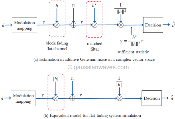
Figure 1: Simulation model for modulation and detection over flat fading channel
Simulation and performance results
In chapter 5 of the book Wireless communication systems in Matlab, the code implementation for complex baseband models for various digital modulators and demodulator are given. The computation and generation of AWGN noise is also given in the book. Using these models, we can create a unified simulation for code for simulating the performance of various modulation techniques over Rician flat-fading channel the simulation model shown in Figure 1(b).
An unified approach is employed to simulate the performance of any of the given modulation technique – MPSK, MQAM or MPAM. The simulation code (given in the book) will automatically choose the selected modulation type, performs Monte Carlo simulation, computes symbol error rates and plots them against the theoretical symbol error rate curves. The simulated performance results obtained for various modulations are shown in the Figure 2.
Figure 2: Performance of various modulations over Ricean flat fading channel
Rate this article: Note: There is a rating embedded within this post, please visit this post to rate it.
The phase transition properties of the different variants of QPSK schemes and MSK, are easily investigated using constellation diagram. Let’s demonstrate how to plot the signal space constellations, for the various modulations used in the transmitter.
Typically, in practical applications, the baseband modulated waveforms are passed through a pulse shaping filter for combating the phenomenon of intersymbol interference (ISI). The goal is to plot the constellation plots of various pulse-shaped baseband waveforms of the QPSK, O-QPSK and π/4-DQPSK schemes. A variety of pulse shaping filters are available and raised cosine filter is specifically chosen for this demo. The raised cosine (RC) pulse comes with an adjustable transition band roll-off parameter α, using which the decay of the transition band can be controlled.
The RC pulse shaping function is expressed in frequency domain as
Equivalently, in time domain, the impulse response corresponds to
A simple evaluation of the equation (2) produces singularities (undefined points) at p(t = 0) and p(t = ±Tsym/(2α)). The value of the raised cosine pulse at these singularities can be obtained by applying L’Hospital’s rule [1] and the values are
The function is then tested. It generates a raised cosine pulse for the given symbol duration Tsym = 1s and plots the time-domain view and the frequency response as shown in Figure 1. From the plot, it can be observed that the RC pulse falls off at the rate of 1/|t|3 as t→∞, which is a significant improvement when compared to the decay rate of a sinc pulse which is 1/|t|. It satisfies Nyquist criterion for zero ISI – the pulse hits zero crossings at desired sampling instants. The transition bands in the frequency domain can be made gradual (by controlling α) when compared to that of a sinc pulse.
Figure 1: Raised-cosine pulse and its manifestation in frequency domain
Plotting constellation diagram
Now that we have constructed a function for raised cosine pulse shaping filter, the next step is to generate modulated waveforms (using QPSK, O-QPSK and π/4-DQPSK schemes), pass them through a raised cosine filter having a roll-off factor, say α = 0.3 and finally plot the constellation. The constellation for MSK modulated waveform is also plotted.
The resulting simulated plot is shown in the Figure 2. From the resulting constellation diagram, following conclusions can be reached.
Conventional QPSK has 180° phase transitions and hence it requires linear amplifiers with high Q factor
The phase transitions of Offset-QPSK are limited to 90° (the 180° phase transitions are eliminated)
The signaling points for π/4-DQPSK is toggled between two sets of QPSK constellations that are shifted by 45° with respect to each other. Both the 90° and 180° phase transitions are absent in this constellation. Therefore, this scheme produces the lower envelope variations than the rest of the two QPSK schemes.
MSK is a continuous phase modulation, therefore no abrupt phase transition occurs when a symbol changes. This is indicated by the smooth circle in the constellation plot. Hence, a band-limited MSK signal will not suffer any envelope variation, whereas, the rest of the QPSK schemes suffer varied levels of envelope variations, when they are band-limited.
The goal of timing recovery is to estimate and correct the sampling instants and phase at the receiver, such that it allows the receiver to decode the transmitted symbols reliably.
What is Symbol timing Recovery :
When transmitting data across a communication system, three things are important: frequency of transmission, phase information and the symbol rate.
In coherent detection/demodulation, both the transmitter and receiver posses the knowledge of exact symbol sampling timing and symbol phase (and/or symbol frequency). While everything is set at the transmitter, the receiver is at the mercy of recovery algorithms to regenerate these information from the incoming signal itself. If the transmission is a passband transmission, the carrier recovery algorithm also recovers the carrier frequency. For phase sensitive systems like BPSK, QPSK etc.., the carrier recovery algorithm recovers the symbol phase so that it is synchronous with the transmitted symbol.
The first part in such a receiver architecture of a MPSK transmitting system is multiplying the incoming signal with sine and cosine components of the carrier wave.
The sine and cosine components are generated using a carrier recovery block (Phase Lock Loop (PLL) or setting a local oscillator to track the variations).
Once the in-phase and quadrature signals are separated out properly, the next task is to match each symbol with the transmitted pulse shape such that the overall SNR of the system improves.
Implementing this in digital domain, the architecture described so far would look like this (Note: the subscript of the incoming signal has changed from analog domain to digital domain – i.e. to )
In the digital architecture above, the matched filter is implemented as a simple finite impulse response (FIR) filter whose impulse response is matched to that of the transmitter pulse shape. It helps the receiver in timing recovery and also it improves the overall SNR of the system by suppressing some amount of noise. The incoming signal up to the point before the matched filter, may have fluctuations in the amplitude. The matched filter also behaves like an averaging filter that smooths out the variations in the signal.
Note that in this digital version, the incoming signal is already a sampled signal. It has already passed through an analog to digital converter that sampled the signal at some sampling rate. From the symbol perspective, the symbols have to be sampled at optimum sampling instant to extract its content properly.
This requires a re-sampler, which resamples the averaged signal at the optimum sampling instant. If the original sampling instant is before or after the optimum sampling point, the timing recovery signal will help to re-sample (re-adjust sampling times) accordingly.
An alternate data pattern (symbols) – [+1,-1,+1,+1,\cdots,] is transmitted across the channel. Assume that each symbol occupies Tsym=8 sample time.
clear all; clc;
n=10; %Number of data symbols
Tsym=8; %Symbol time interms of sample time or oversampling rate equivalently
%data=2*(rand(n,1)<0.5)-1;
data=[1 -1 1 -1 1 -1 1 -1 1 -1]'; %BPSK data
bpsk=reshape(repmat(data,1,Tsym)',n*Tsym,1); %BPSK signal

figure('Color',[1 1 1]);
subplot(3,1,1);
plot(bpsk);
title('Ideal BPSK symbols');
xlabel('Sample index [n]');
ylabel('Amplitude')
set(gca,'XTick',0:8:80);
axis([1 80 -2 2]); grid on;
Lets add white gaussian noise (awgn). A random noise of standard deviation 0.25 is generated and added with the generated BPSK symbols.
noise=0.25*randn(size(bpsk)); %Adding some amount of noise
received=bpsk+noise; %Received signal with noise

subplot(3,1,2);
plot(received);
title('Transmitted BPSK symbols (with noise)');
xlabel('Sample index [n]');
ylabel('Amplitude')
set(gca,'XTick',0:8:80);
axis([1 80 -2 2]); grid on;
From the first plot, we see that the transmitted pulse is a rectangular pulse that spans Tsym samples. In the illustration, Tsym=8. The best averaging filter (matched filter) for this case is a rectangular filter (though they are not preferred in practice, I am just using it for simplifying the illustration) that spans 8 samples. Such a rectangular pulse can be mathematically represented in terms of unit step function as
The resulting rectangular pulse will have a value of 0.5 at the edges of the sampling instants (index 0 and 7) and a value of ‘1’ at the remaining indices in between the edges. Such a rectangular function is indicated below.
The incoming signal is convolved with the averaging filter and the resultant output is given below
We can note that the averaged output peaks at the locations where the symbol transition occurs. Thus, when the signal is sampled at those ideal locations, the BPSK symbols [+1,-1,+1, …] can be recovered perfectly.
But the problem here is: “How does the receiver know the ideal sampling instants?”. The solution is “someone has to supply those ideal sampling instants”. A symbol time recovery circuit is used for this purpose.
Coming back to the receiver architecture, lets add a symbol time recovery circuit that supplies the recovered timing instants. The signal will be re-sampled at those instants supplied by the recovery circuit.
The Algorithm behind Symbol Timing Recovery:
Different algorithms exist for symbol timing recovery and synchronization. An “Early/Late Symbol Recovery algorithm” is illustrated here.
The algorithm starts by selecting an arbitrary sample at some time (denoted by T). It captures the two adjacent samples (on either side of the sampling instant T) that are separated by δ seconds. The sample at the index T-δ is called Early Sample and the sample at the index T+δ is called Late Sample. The timing error is generated by comparing the amplitudes of the early and late samples. The next symbol sampling time instant is either advanced or delayed based on the sign of difference between the early and late sample.
1) If the Early Sample = Late Sample : The peak occurs at the on-time sampling instant T. No adjustment in the timing is needed. 2) If |Early Sample| > |Late Sample| : Late timing, the sampling time is offset so that the next symbol is sampled T-δ/2 seconds after the current sampling time. 3) If |Early Sample| < |Late Sample| : Early timing, the sampling time is offset so that the next symbol is sampled T+δ/2 seconds after the current sampling time.
These three situations are shown next.
There exist many variations to the above mentioned algorithm. The Early/Late synchronization technique given here is the simplest one taken for illustration.
Let’s complete the architecture with a signal quantization and constellation de-mapping block which gives out the estimated demodulated symbols.
Rate this article: Note: There is a rating embedded within this post, please visit this post to rate it.
Quadrature Phase Shift Keying (QPSK) is a form of phase modulation technique, in which two information bits (combined as one symbol) are modulated at once, selecting one of the four possible carrier phase shift states.
Figure 1: Waveform simulation model for QPSK modulation
The QPSK signal within a symbol duration \(T_{sym}\) is defined as
\[s(t) = A \cdot cos \left[2 \pi f_c t + \theta_n \right], \quad \quad 0 \leq t \leq T_{sym},\; n=1,2,3,4 \quad \quad (1) \]
Therefore, the four possible initial signal phases are \(\pi/4, 3 \pi/4, 5 \pi/4\) and \(7 \pi/4\) radians. Equation (1) can be re-written as
\[\begin{align} s(t) &= A \cdot cos \theta_n \cdot cos \left( 2 \pi f_c t\right) – A \cdot sin \theta_n \cdot sin \left( 2 \pi f_c t\right) \\ &= s_{ni} \phi_i(t) + s_{nq} \phi_q(t) \quad\quad \quad \quad \quad\quad \quad \quad \quad\quad \quad \quad \quad\quad \quad \quad (3) \end{align} \]
The above expression indicates the use of two orthonormal basis functions: \( \left\langle \phi_i(t),\phi_q(t)\right\rangle\) together with the inphase and quadrature signaling points: \( \left\langle s_{ni}, s_{nq}\right\rangle\). Therefore, on a two dimensional co-ordinate system with the axes set to \( \phi_i(t)\) and \(\phi_q(t)\), the QPSK signal is represented by four constellation points dictated by the vectors \(\left\langle s_{ni}, s_{nq}\right\rangle\) with \( n=1,2,3,4\).
The QPSK transmitter, shown in Figure 1, is implemented as a matlab function qpsk_mod. In this implementation, a splitter separates the odd and even bits from the generated information bits. Each stream of odd bits (quadrature arm) and even bits (in-phase arm) are converted to NRZ format in a parallel manner.
function [s,t,I,Q] = qpsk_mod(a,fc,OF)
%Modulate an incoming binary stream using conventional QPSK
%a - input binary data stream (0's and 1's) to modulate
%fc - carrier frequency in Hertz
%OF - oversampling factor (multiples of fc) - at least 4 is better
%s - QPSK modulated signal with carrier
%t - time base for the carrier modulated signal
%I - baseband I channel waveform (no carrier)
%Q - baseband Q channel waveform (no carrier)
L = 2*OF;%samples in each symbol (QPSK has 2 bits in each symbol)
ak = 2*a-1; %NRZ encoding 0-> -1, 1->+1
I = ak(1:2:end);Q = ak(2:2:end);%even and odd bit streams
I=repmat(I,1,L).'; Q=repmat(Q,1,L).';%even/odd streams at 1/2Tb baud
I = I(:).'; Q = Q(:).'; %serialize
fs = OF*fc; %sampling frequency
t=0:1/fs:(length(I)-1)/fs; %time base
iChannel = I.*cos(2*pi*fc*t);qChannel = -Q.*sin(2*pi*fc*t);
s = iChannel + qChannel; %QPSK modulated baseband signal
The timing diagram for BPSK and QPSK modulation is shown in Figure 2. For BPSK modulation the symbol duration for each bit is same as bit duration, but for QPSK the symbol duration is twice the bit duration: \(T_{sym}=2T_b\). Therefore, if the QPSK symbols were transmitted at same rate as BPSK, it is clear that QPSK sends twice as much data as BPSK does. After oversampling and pulse shaping, it is intuitively clear that the signal on the I-arm and Q-arm are BPSK signals with symbol duration \(2T_b\). The signal on the in-phase arm is then multiplied by \(cos (2 \pi f_c t)\) and the signal on the quadrature arm is multiplied by \(-sin (2 \pi f_c t)\). QPSK modulated signal is obtained by adding the signal from both in-phase and quadrature arms.
Note: The oversampling rate for the simulation is chosen as \(L=2 f_s/f_c\), where \(f_c\) is the given carrier frequency and \(f_s\) is the sampling frequency satisfying Nyquist sampling theorem with respect to the carrier frequency (\(f_s \geq f_c\)). This configuration gives integral number of carrier cycles for one symbol duration.
Figure 2: Timing diagram for BPSK and QPSK modulations
The receiver
Due to its special relationship with BPSK, the QPSK receiver takes the simplest form as shown in Figure 3. In this implementation, the I-channel and Q-channel signals are individually demodulated in the same way as that of BPSK demodulation. After demodulation, the I-channel bits and Q-channel sequences are combined into a single sequence. The function qpsk_demod implements a QPSK demodulator as per Figure 3.
Read more about QPSK, implementation of their modulator and demodulator, performance simulation in these books:
Figure 3: Waveform simulation model for QPSK demodulation
Performance simulation over AWGN
The complete waveform simulation for the aforementioned QPSK modulation and demodulation is given next. The simulation involves, generating random message bits, modulating them using QPSK modulation, addition of AWGN channel noise corresponding to the given signal-to-noise ratio and demodulating the noisy signal using a coherent QPSK receiver. The waveforms at the various stages of the modulator are shown in the Figure 4.
Figure 4: Simulated QPSK waveforms at the transmitter side
The performance simulation for the QPSK transmitter-receiver combination was also coded in the code given above and the resulting bit-error rate performance curve will be same as that of conventional BPSK. A QPSK signal essentially combines two orthogonally modulated BPSK signals. Therefore, the resulting performance curves for QPSK – \(E_b/N_0\) Vs. bits-in-error – will be same as that of conventional BPSK.
QPSK variants
QPSK modulation has several variants, three such flavors among them are: Offset QPSK, π/4-QPSK and π/4-DQPSK.
Offset-QPSK
Offset-QPSK is essentially same as QPSK, except that the orthogonal carrier signals on the I-channel and the Q-channel are staggered (one of them is delayed in time). In OQPSK, the orthogonal components cannot change states at the same time, this is because the components change state only at the middle of the symbol periods (due to the half symbol offset in the Q-channel). This eliminates 180° phase shifts all together and the phase changes are limited to 0° or 90° every bit period.
Elimination of 180° phase shifts in OQPSK offers many advantages over QPSK. Unlike QPSK, the spectrum of OQPSK remains unchanged when band-limited [1]. Additionally, OQPSK performs better than QPSK when subjected to phase jitters [2]. Further improvements to OQPSK can be obtained if the phase transitions are avoided altogether – as evident from continuous modulation schemes like Minimum Shift Keying (MSK) technique.
π/4-QPSK and π/4-DQPSK
In π/4-QPSK, the signaling points of the modulated signals are chosen from two QPSK constellations that are just shifted π/4 radians (45°) with respect to each other. Switching between the two constellations every successive bit ensures that the phase changes are confined to odd multiples of 45°. Therefore, phase transitions of 90° and 180° are eliminated.
π/4-QPSK preserves the constant envelope property better than QPSK and OQPSK. Unlike QPSK and OQPSK schemes, π/4-QPSK can be differentially encoded, therefore enabling the use of both coherent and non-coherent demodulation techniques. Choice of non-coherent demodulation results in simpler receiver design. Differentially encoded π/4-QPSK is referred as π/4-DQPSK.
Read more about QPSK and its variants, implementation of their modulator and demodulator, performance simulation in these books:
This website uses cookies to improve your experience while you navigate through the website. Out of these, the cookies that are categorized as necessary are stored on your browser as they are essential for the working of basic functionalities of the website. We also use third-party cookies that help us analyze and understand how you use this website. These cookies will be stored in your browser only with your consent. You also have the option to opt-out of these cookies. But opting out of some of these cookies may affect your browsing experience.
Necessary cookies are absolutely essential for the website to function properly. These cookies ensure basic functionalities and security features of the website, anonymously.
Cookie
Duration
Description
cookielawinfo-checbox-analytics
11 months
This cookie is set by GDPR Cookie Consent plugin. The cookie is used to store the user consent for the cookies in the category "Analytics".
cookielawinfo-checbox-analytics
11 months
This cookie is set by GDPR Cookie Consent plugin. The cookie is used to store the user consent for the cookies in the category "Analytics".
cookielawinfo-checbox-functional
11 months
The cookie is set by GDPR cookie consent to record the user consent for the cookies in the category "Functional".
cookielawinfo-checbox-functional
11 months
The cookie is set by GDPR cookie consent to record the user consent for the cookies in the category "Functional".
cookielawinfo-checbox-others
11 months
This cookie is set by GDPR Cookie Consent plugin. The cookie is used to store the user consent for the cookies in the category "Other.
cookielawinfo-checbox-others
11 months
This cookie is set by GDPR Cookie Consent plugin. The cookie is used to store the user consent for the cookies in the category "Other.
cookielawinfo-checkbox-necessary
11 months
This cookie is set by GDPR Cookie Consent plugin. The cookies is used to store the user consent for the cookies in the category "Necessary".
cookielawinfo-checkbox-performance
11 months
This cookie is set by GDPR Cookie Consent plugin. The cookie is used to store the user consent for the cookies in the category "Performance".
viewed_cookie_policy
11 months
The cookie is set by the GDPR Cookie Consent plugin and is used to store whether or not user has consented to the use of cookies. It does not store any personal data.
Functional cookies help to perform certain functionalities like sharing the content of the website on social media platforms, collect feedbacks, and other third-party features.
Performance cookies are used to understand and analyze the key performance indexes of the website which helps in delivering a better user experience for the visitors.
Analytical cookies are used to understand how visitors interact with the website. These cookies help provide information on metrics the number of visitors, bounce rate, traffic source, etc.


![y[n]](https://s0.wp.com/latex.php?latex=y%5Bn%5D&bg=ffffff&fg=000&s=0&c=20201002)


![u[n]-u[n-8]](https://s0.wp.com/latex.php?latex=u%5Bn%5D-u%5Bn-8%5D+&bg=ffffff&fg=000&s=2&c=20201002)


