Shannon limit on power efficiency – demystified

The Shannon power efficiency limit is the limit of a band-limited system irrespective of modulation or coding scheme. It informs us the minimum required energy per bit required at the transmitter for reliable communication. It is also called unconstrained Shannon power efficiency Limit. If we select a particular modulation scheme or an encoding scheme, we calculate the constrained Shannon limit for that scheme.

Before proceeding, I urge you to go through the fundamentals of Shannon Capacity theorem in this article.

This article is part of the book
Wireless Communication Systems in Matlab (second edition), ISBN: 979-8648350779 available in ebook (PDF) format and Paperback (hardcopy) format.

Channel capacity and power efficiency

One of the objective of a communication system design is to reliably send information at the lowest possible power level. The system should be able to provide acceptable bit-error-rate (BER) performance at the lowest possible power level. Often, this performance is charted in terms of BER Vs. . The quantity is called power efficiency, denoted as . Power efficiency is defined as the ratio of signal energy per bit () to noise power spectral density per bit ( – required at the receiver input to achieve certain BER.

From equations (1) and (2) shown in this post, the condition for reliable transmission through a channel is given by

Re-writing in terms of spectral efficiency , the Shannon limit on power efficiency for reliable communication is given by

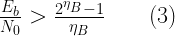
With this equation, we can calculate the minimum required to achieve a certain spectral efficiency. As an example, lets simulate and plot the relationship between and spectral efficiency , as given in equation (3).

k =0.1:0.001:15; EbN0=(2.ˆk-1)./k;
semilogy(10*log10(EbN0),k);
xlabel('E_b/N_o (dB)');ylabel('Spectral Efficiency (\eta)');
title('Channel Capacity & Power efficiency limit')
hold on;grid on; xlim([-2 20]);ylim([0.1 10]);
yL = get(gca,'YLim');
line([-1.59 -1.59],yL,'Color','r','LineStyle','--');

The ultimate Shannon limit

From the plot in Fig. 1, we notice that the Shannon limit on is a monotonic function of . When , the Shannon limit on is equal to . If , the limit is at . When , the Shannon limit on approaches . This value is called ultimate Shannon limit or specifically absolute Shannon power efficiency limit. This limit informs us the minimum required energy per bit required at the transmitter for reliable communication. It is one among the important measures in designing a coding scheme.

Shannon power efficiency limit
Figure 1: Shannon Power Efficiency Limit

The ultimate Shannon limit can be derived using L’Hospital’s rule as follows. The asymptotic value, , that we are seeking, is the value of as the spectral efficiency approaches .

Let and . As and the argument of the limit becomes indeterminate (), L’Hospital’s rule can be applied in this case. According to L’Hospital’s rule, if and are both zero or are both , then for any value of .

Thus, the next step boils down to finding the first derivative of and . Expressing in natural logarithm.


Let and , then by chain rule of differentiation,

Since , the first derivative of is

Using equations (8) and (9), and applying L’Hospital’s rule, the Shannon’s limit on is given by

Unconstrained and constrained Shannon limit

The absolute Shannon power efficiency limit is the limit of a band-limited system irrespective of modulation or coding scheme. This is also called unconstrained Shannon power efficiency Limit. If we select a particular modulation scheme or an encoding scheme, we calculate the constrained Shannon limit for that scheme.

Shannon power efficiency limit does not depend on error probability. Shannon limit tells us the minimum possible required for achieving an arbitrarily small probability of error as , where is the number of signaling levels for the modulation technique, for BPSK , QPSK and so on. It gives the minimum possible that satisfies the Shannon theorem. In other words, it gives the minimum possible required to achieve maximum transmission capacity ( , where, is the rate of transmission and is the channel capacity). It will not specify error probability at that limit. Nor will it give any direction on coding technique that can be used to achieve that limit. As the capacity is approached, the system complexity will increase drastically. So the aim of any system design is to achieve that limit. For example, the error probability performances of Turbo codes are very close to Shannon limit [1].

As an example, let’s evaluate the performance of a 2-PAM (Pulse Amplitude Modulation) system and determine the maximum possible coding gain that can be achieved by the most advanced coding scheme. The methodology for simulating the performance of a 2-PAM system is described in chapter 5 and 6. Using this methodology, the performance of a 2-PAM system is simulated and plotted in Figure 2. The absolute Shannon power efficiency limits when the spectral efficiency is and are also referenced on the plot.

The spectral efficiency of an ideal 2-PAM system is . Hence, if the target bit error rate is , then a coding gain of can be achieved using powerful codes, if we have to maintain the nominal spectral efficiency at .

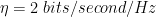
If there is no limit on the spectral efficiency, then we can let . In this case, the absolute Shannon power efficiency limit is when . Thus a coding gain of approximately is possible with powerful codes if we let the spectral efficiency approach zero.

Rate this article: Note: There is a rating embedded within this post, please visit this post to rate it.

References

[1] C. Berrou, A. Glavieux, and P. Thitimajshima, Near Shannon limit error-correcting coding and decoding: Turbocodes, IEEE Int. Conf. on Comm., (ICC ’93), 2:1064-1070, May 1993.↗

 Related topics in this chapter

Introduction
Shannon’s noisy channel coding theorem
Unconstrained capacity for bandlimited AWGN channel
● Shannon’s limit on spectral efficiency
Shannon’s limit on power efficiency
● Generic capacity equation for discrete memoryless channel (DMC)
 □ Capacity over binary symmetric channel (BSC)
 □ Capacity over binary erasure channel (BEC)
● Constrained capacity of discrete input continuous output memoryless AWGN channel
● Ergodic capacity over a fading channel

Books by the author


Wireless Communication Systems in Matlab
Second Edition(PDF)

Note: There is a rating embedded within this post, please visit this post to rate it.
Checkout Added to cart

Digital Modulations using Python
(PDF ebook)

Note: There is a rating embedded within this post, please visit this post to rate it.
Checkout Added to cart

Digital Modulations using Matlab
(PDF ebook)

Note: There is a rating embedded within this post, please visit this post to rate it.
Checkout Added to cart
Hand-picked Best books on Communication Engineering
Best books on Signal Processing

Capacity of MIMO system over fading Channels

As reiterated in the previous article, a MIMO system is used to increase the capacity dramatically and also to improve the quality of a communication link. Increased capacity is obtained by spatial multiplexing and increased quality is obtained by diversity techniques (Space time coding). Capacity of MIMO system over a variety of channels (AWGN, fading channels) is of primary importance. It is desirable to know the capacity improvements offered by a MIMO system over the conventional SISO system. The capacity equations for a conventional SISO system over AWGN and fading channels were discussed in the earlier articles. As a per-requisite, readers are encouraged to go through the detailed discussion on channel capacity and Shannon’s Theorem too.

For those who are directly jumping here (without reading the article on SISO channel capacity), a few definitions are given below.

Entropy

The average amount of information per symbol (measured in bits/symbol) is called Entropy. Given a set of N discrete information symbols – represented as random variable having probabilities denoted by a Probability Mass Function , the entropy of X is given by

Entropy is a measure of uncertainty of a random variable , therefore reflects the amount of information required on an average to describe the random variable. In general, it has the following bounds

Entropy hits the lower bound of zero (no uncertainty, therefore no information) for a completely deterministic system (probability of correct transmission ). It reaches the upper bound when the input symbols are equi-probable.

Capacity and mutual information

Following figure represents a discrete memory less (noise term corrupts the input symbols independently) channel, where the input and output are represented as random variables and respectively. Statistically, such a channel can be expressed by transition or conditional probabilities. That is, given a set of inputs to the channel, the probability of observing the output of the channel is expressed as conditional probability

For such a channel, the mutual information denotes the amount of information that one random variable contains about the other random variable

is the amount of information in before observing and thus the above quantity can be seen as the reduction of uncertainty of from the observation of .

The information capacity C is obtained by maximizing this mutual information taken over all possible input distributions p(x) [1].

MIMO flat fading Channel model

A MIMO system over a flat fading channel can be represented in the complex baseband notation.

where,
– received response from the channel – dimension
– the complex channel matrix of dimension
– vector representing transmitted signal – dimension . Assuming Gaussian signals i.e, , where is the covariance matrix of the transmit vector
– the number of transmit antennas
– the number of receive antennas
– complex baseband additive white Gaussian noise vector of dimension . It is assumed that the noise is spatially white  where is the covariance matrix of noise.

Note: The trace of the covariance matrix of the transmit vector gives the average transmit power, , where is the transmit power constraint applied at the transmitter.

Signal Covariance Matrices

It was assumed that the input signal vector and the noise vector  are uncorrelated. Therefore, the covariance matrix of the received signal vector is given by

In the above equation, the operator on the matrices denote Hermitian transpose operation. Thus, there are three covariance matrix involved here

  – Covariance matrix of input signal vector
– Covariance matrix of channel response vector
– Covariance matrix of noise vector

Channel State Information

The knowledge of the channel matrix , at the transmitter is called Channel State Information at the Transmitter (CSIT). If the receiver knows about the present state of the channel matrix, that knowledge is called Channel State Information at the Receiver (CSIR). Click here for more information on CSI and another related concept called condition number.

MIMO capacity discussion for CSIT known and unknown cases at the transmitter will be discussed later.

Capacity with transmit power constraint

Now, we would like to evaluate capacity for the most practical scenario, where the average power, given by , that can be expensed at the transmitter is limited to . Thus, the channel capacity is now constrained by this average transmit power, given as

For the further derivations, we assume that the receiver possesses perfect knowledge about the channel. Furthermore, we assume that the input random variable X is independent of the noise N and the noise vector is zero mean Gaussian distributed with covariance matrix   -i.e, .

Note that both the input symbols in the vector and the output symbols in the vector take continuous values upon transmission and reception and the values are discrete in time (Continuous input Continuous output discrete Memoryless Channel – CCMC). For such continuous random variable, differential entropy – is considered. Expressing the mutual information in terms of differential entropy,

Since it is assumed that the channel is perfectly known at the receiver, the uncertainty of the channel h conditioned on X is zero, i.e, . Furthermore, it is assumed that the noise is independent of the input , i.e, . Thus, the mutual information is

Following the procedure laid out here, the differential entropy is calculated as

Using \((6)\) and the similar procedure for calculating above , The differential entropy is given by

Substituting equations (10) and (11) in (9), the capacity is given by

For the case, where the noise is uncorrelated (spatially white) between the antenna branches, , where  is the identity matrix of dimension .

Thus the capacity for MIMO flat fading channel can be written as

The capacity equation (13) contains random variables, and therefore the capacity will also be random. For obtaining meaningful result, for fading channels two different capacities can be defined.

If the CSIT is **UNKNOWN** at the transmitter, it is optimal to evenly distribute the available transmit power at the transmit antennas. That is, , where is the identity matrix of dimension .

Ergodic Capacity

Ergodic capacity is defined as the statistical average of the mutual information, where the expectation is taken over 

Outage Capacity

Defined as the information rate below which the instantaneous mutual information falls below a prescribed value of probability expressed as percentage – q.

A word on capacity of a MIMO system over AWGN Channels

The capacity of MIMO system over AWGN channel can be derived in a very similar manner. The only difference will be the channel matrix. For the AWGN channel, the channel matrix will be a constant. The final equation for capacity will be very similar and will follow the lines of capacity of SISO over AWGN channel.

Rate this article: Note: There is a rating embedded within this post, please visit this post to rate it.

References:

[1] Andrea J. Goldsmith & Pravin P. Varaiya, Capacity, mutual information, and coding for finite-state Markov channels,IEEE Transactions on Information Theory, Vol 42, No.3, May 1996.↗

Articles in this series
[1] Introduction to Multiple Antenna Systems
[2] MIMO - Diversity and Spatial Multiplexing
[3] Characterizing a MIMO channel - Channel State Information (CSI) and Condition number
[4] Capacity of a SISO system over a fading channel
[5] Ergodic Capacity of a SISO system over a Rayleigh Fading channel - Simulation in Matlab
[6] Capacity of a MIMO system over Fading Channels
[7] Single Input Multiple Output (SIMO) models for receive diversity
[8] Receiver diversity - Selection Combining
[9] Receiver diversity – Maximum Ratio Combining (MRC)

Books by the author


Wireless Communication Systems in Matlab
Second Edition(PDF)

Note: There is a rating embedded within this post, please visit this post to rate it.
Checkout Added to cart

Digital Modulations using Python
(PDF ebook)

Note: There is a rating embedded within this post, please visit this post to rate it.
Checkout Added to cart

Digital Modulations using Matlab
(PDF ebook)

Note: There is a rating embedded within this post, please visit this post to rate it.
Checkout Added to cart
Hand-picked Best books on Communication Engineering
Best books on Signal Processing

Ergodic Capacity of SISO flat fading channel

Understand ergodic capacity of a SISO flat-fading system over fading channels. Model and simulate capacity curves in Matlab.

Channel model

In the previous post, derivation of SISO fading channel capacity was discussed. For a flat fading channel (model shown below), with the perfect knowledge of the channel at the receiver, the capacity of a SISO link was derived as

where,  is flat fading complex channel impulse response that is held constant for each block of transmitted symbols, is the average input power at the transmit antenna, is the signal-to-noise ratio (SNR) at the receiver input and is the noise power of the channel.

Figure 1: A frequency-flat channel model

Since the channel impulse response is a random variable, the channel capacity equation shown above is also random. To circumvent this, Ergodic channel capacity was defined along with outage capacity. The Ergodic channel capacity is defined as the statistical average of the mutual information, where the expectation is taken over

Jensen’s inequality [1] states that for any concave function f(x), where x is a random variable,

Applying Jensen’s inequality to Ergodic capacity in equation (2),

This implies that the Ergodic capacity of a fading channel cannot exceed that of an AWGN channel with constant gain. The above equation is simulated in Matlab for a Rayleigh Fading channel with and the plots are shown below.

Matlab code

%This work is licensed under a Creative Commons
%Attribution-NonCommercial-ShareAlike 4.0 International License
%Attribute author : Mathuranathan Viswanathan at gaussianwaves.com
snrdB=-10:0.5:20; %Range of SNRs to simulate

h= (randn(1,100) + 1i*randn(1,100) )/sqrt(2); %Rayleigh flat channel
sigma_z=1; %Noise power - assumed to be unity


snr = 10.^(snrdB/10); %SNRs in linear scale
P=(sigma_z^2)*snr./(mean(abs(h).^2)); %Calculate corresponding values for P

C_erg_awgn= (log2(1+ mean(abs(h).^2).*P/(sigma_z^2))); %AWGN channel capacity (Bound)
C_erg = mean((log2(1+ ((abs(h).^2).')*P/(sigma_z^2)))); %ergodic capacity for Fading channel

plot(snrdB,C_erg_awgn,'b'); hold on;
plot(snrdB,C_erg,'r'); grid on;
legend('AWGN channel capacity','Fading channel Ergodic capacity');
title('SISO fading channel - Ergodic capacity');
xlabel('SNR (dB)');ylabel('Capacity (bps/Hz)');
Figure 2: Simulated capacity curves for SISO flat-fading channel

Rate this article: Note: There is a rating embedded within this post, please visit this post to rate it.

References

[1] Konstantinos G. Derpanis, Jensen’s Inequality, Version 1.0,March 12, 2005.↗

Articles in this series
[1] Introduction to Multiple Antenna Systems
[2] MIMO - Diversity and Spatial Multiplexing
[3] Characterizing a MIMO channel - Channel State Information (CSI) and Condition number
[4] Capacity of a SISO system over a fading channel
[5] Ergodic Capacity of a SISO system over a Rayleigh Fading channel - Simulation in Matlab
[6] Capacity of a MIMO system over Fading Channels
[7] Single Input Multiple Output (SIMO) models for receive diversity
[8] Receiver diversity - Selection Combining
[9] Receiver diversity – Maximum Ratio Combining (MRC)

Books by the author


Wireless Communication Systems in Matlab
Second Edition(PDF)

Note: There is a rating embedded within this post, please visit this post to rate it.
Checkout Added to cart

Digital Modulations using Python
(PDF ebook)

Note: There is a rating embedded within this post, please visit this post to rate it.
Checkout Added to cart

Digital Modulations using Matlab
(PDF ebook)

Note: There is a rating embedded within this post, please visit this post to rate it.
Checkout Added to cart
Hand-picked Best books on Communication Engineering
Best books on Signal Processing

Capacity of SISO system over a fading channel

As reiterated in the previous article, a MIMO system is used to increase the capacity dramatically and also to improve the quality of a communication link. Increased capacity is obtained by spatial multiplexing and increased quality is obtained by diversity techniques (Space time coding). Capacity equations of a MIMO system over a variety of channels (AWGN, fading channels) is of primary importance. It is desirable to know the capacity improvements offered by a MIMO system over the capacity of SISO system.

To begin with, we will be looking into the capacity equations for a conventional SISO system over AWGN and fading channels followed by capacity equations for a MIMO systems. As a pre-requisite, readers are encouraged to go through the detailed discussion on channel capacity and Shannon’s Theorem.

To begin with, clarity over few definitions are needed.

Entropy

The average amount of information per symbol (measured in bits/symbol) is called Entropy. Given a set of discrete information symbols – represented as random variable having probabilities denoted by a Probability Mass Function , the entropy of is given by

Entropy is a measure of uncertainty of a random variable , therefore reflects the amount of information required on an average to describe the random variable. In general, it has the following bounds

Entropy hits the lower bound of zero (no uncertainty, therefore no information) for a completely deterministic system (probability of correct transmission ). It reaches the upper bound when the input symbols are equi-probable.

Capacity and mutual information

Following figure represents a discrete memoryless (noise term corrupts the input symbols independently) channel, where the input and output are represented as random variables and respectively. Statistically, such a channel can be expressed by transition or conditional probabilities. That is, given a set of inputs to the channel, the probability of observing the output of the channel is expressed as conditional probability

For such a channel, the mutual information denotes the amount of information that one random variable contains about the other random variable

is the amount of information in before observing and thus the above quantity can be seen as the reduction of uncertainty of from the observation of latex .

The information capacity is obtained by maximizing this mutual information taken over all possible input distributions [1].

SISO fading Channel

A SISO fading channel can be represented as the convolution of the complex channel impulse response (represented as a random variable ) and the input .

Here, is complex baseband additive white Gaussian noise and the above equation is for a single realization of complex output . If the channel is assumed to be flat fading or of block fading type (channel does not vary over a block of symbols), the above equation can be simply written without the convolution operation (refer this article to know how equations (5) & (6) are equivalent for a flat-fading channel).

For different communication fading channels, the channel impulse response can be modeled using various statistical distributions. Some of the common distributions as Rayleigh, Rician, Nakagami-m, etc.,

Capacity with transmit power constraint

Now, we would like to evaluate capacity for the most practical scenario, where the average power, given by , that can be expensed at the transmitter is limited to . Thus, the channel capacity is now constrained by this average transmit power, given as

For the further derivations, we assume that the receiver possesses perfect knowledge about the channel. Furthermore, we assume that the input random variable is independent of the noise and the noise is zero mean Gaussian distributed with variance -i.e, .

Note that both the input symbols and the output symbols take continuous values upon transmission and reception and the values are discrete in time (Continuous input Continuous output discrete Memoryless Channel – CCMC). For such continuous random variable, differential entropy – is considered. Expressing the mutual information in-terms of differential entropy,

Mutual Information and differential entropy

Since it is assumed that the channel is perfectly known at the receiver, the uncertainty of the channel conditioned on is zero, i.e, . Furthermore, it is assumed that the noise is independent of the input , i.e, . Thus, the mutual information is

For a complex Gaussian noise with non-zero mean and variance , the PDF of the noise is given by

The differential entropy for the noise is given by

This shows that the differential entropy is not dependent on the mean of . Therefore, it is immune to translations (shifting of mean value) of the PDF. For the problem of computation of capacity,

and given the differential entropy , the mutual information is maximized by maximizing the differential entropy . The fact is, the Gaussian random variables itself are differential entropy maximizers. Therefore, the mutual information is maximized when the variable is also Gaussian and therefore the differential entropy . Where, the received average power is given by

Thus the capacity is given by

Representing the entire received signal-to-ratio as , the capacity of a SISO system over a fading channel is given by

For the fading channel considered above, the term channel is modeled as a random variable. Thus, the capacity equation above is also a random variable. Thus, for fading channels two different capacities can be defined.

Ergodic Capacity

Ergodic capacity is defined as the statistical average of the mutual information, where the expectation is taken over

Outage Capacity

Defined as the information rate at which the instantaneous mutual information falls below a prescribed value of probability expressed as percentage – .

Continue reading on simulating ergodic capacity of a SISO channel…

Rate this article: Note: There is a rating embedded within this post, please visit this post to rate it.

References:

[1] Andrea J. Goldsmith & Pravin P. Varaiya, Capacity, mutual information, and coding for finite-state Markov channels,IEEE Transactions on Information Theory, Vol 42, No.3, May 1996.↗

Articles in this series
[1] Introduction to Multiple Antenna Systems
[2] MIMO - Diversity and Spatial Multiplexing
[3] Characterizing a MIMO channel - Channel State Information (CSI) and Condition number
[4] Capacity of a SISO system over a fading channel
[5] Ergodic Capacity of a SISO system over a Rayleigh Fading channel - Simulation in Matlab
[6] Capacity of a MIMO system over Fading Channels
[7] Single Input Multiple Output (SIMO) models for receive diversity
[8] Receiver diversity - Selection Combining
[9] Receiver diversity – Maximum Ratio Combining (MRC)

Books by the author


Wireless Communication Systems in Matlab
Second Edition(PDF)

Note: There is a rating embedded within this post, please visit this post to rate it.
Checkout Added to cart

Digital Modulations using Python
(PDF ebook)

Note: There is a rating embedded within this post, please visit this post to rate it.
Checkout Added to cart

Digital Modulations using Matlab
(PDF ebook)

Note: There is a rating embedded within this post, please visit this post to rate it.
Checkout Added to cart
Hand-picked Best books on Communication Engineering
Best books on Signal Processing

Shannon theorem – demystified

Shannon theorem dictates the maximum data rate at which the information can be transmitted over a noisy band-limited channel. The maximum data rate is designated as channel capacity. The concept of channel capacity is discussed first, followed by an in-depth treatment of Shannon’s capacity for various channels.

Introduction

The main goal of a communication system design is to satisfy one or more of the following objectives.

● The transmitted signal should occupy smallest bandwidth in the allocated spectrum – measured in terms of bandwidth efficiency also called as spectral efficiency – \(\eta_B\).
● The designed system should be able to reliably send information at the lowest practical power level. This is measured in terms of power efficiency – \(\eta_P\).
● Ability to transfer data at higher rates – \(R\) bits=second.
● The designed system should be robust to multipath effects and fading.
● The system should guard against interference from other sources operating in the same frequency – low carrier-to-cochannel signal interference ratio (CCI).
● Low adjacent channel interference from near by channels – measured in terms of adjacent channel Power ratio (ACPR).
● Easier to implement and lower operational costs.

Chapter 2 in my book ‘Wireless Communication systems in Matlab’, is intended to describe the effect of first three objectives when designing a communication system for a given channel. A great deal of information about these three factors can be obtained from Shannon’s noisy channel coding theorem.

Shannon’s noisy channel coding theorem

For any communication over a wireless link, one must ask the following fundamental question: What is the optimal performance achievable for a given channel ?. The performance over a communication link is measured in terms of capacity, which is defined as the maximum rate at which the information can be transmitted over the channel with arbitrarily small amount of error.

It was widely believed that the only way for reliable communication over a noisy channel is to reduce the error probability as small as possible, which in turn is achieved by reducing the data rate. This belief was changed in 1948 with the advent of Information theory by Claude E. Shannon. Shannon showed that it is in fact possible to communicate at a positive rate and at the same time maintain a low error probability as desired. However, the rate is limited by a maximum rate called the channel capacity. If one attempts to send data at rates above the channel capacity, it will be impossible to recover it from errors. This is called Shannon’s noisy channel coding theorem and it can be summarized as follows:

● A given communication system has a maximum rate of information – C, known as the channel capacity.
● If the transmission information rate R is less than C, then the data transmission in the presence of noise can be made to happen with arbitrarily small error probabilities by using intelligent coding techniques.
● To get lower error probabilities, the encoder has to work on longer blocks of signal data. This entails longer delays and higher computational requirements.

The theorem indicates that with sufficiently advanced coding techniques, transmission that nears the maximum channel capacity – is possible with arbitrarily small errors. One can intuitively reason that, for a given communication system, as the information rate increases, the number of errors per second will also increase.

Shannon’s noisy channel coding theorem is a generic framework that can be applied to specific scenarios of communication. For example, communication through a band-limited channel in presence of noise is a basic scenario one wishes to study. Therefore, study of information capacity over an AWGN (additive white gaussian noise) channel provides vital insights, to the study of capacity of other types of wireless links, like fading channels.

Unconstrained capacity for band-limited AWGN channel

Real world channels are essentially continuous in both time as well as in signal space. Real physical channels have two fundamental limitations : they have limited bandwidth and the power/energy of the input signal to such channels is also limited. Therefore, the application of information theory on such continuous channels should take these physical limitations into account. This will enable us to exploit such continuous channels for transmission of discrete information.

In this section, the focus is on a band-limited real AWGN channel, where the channel input and output are real and continuous in time. The capacity of a continuous AWGN channel that is bandwidth limited to \(B\) Hz and average received power constrained to \(P\) Watts, is given by

\[C_{awgn} \left( P,B\right) = B\; log_2 \left( 1 + \frac{P}{N_0 B}\right) \quad bits/s \quad\quad (1)\]

Here, \(N_0/2\) is the power spectral density of the additive white Gaussian noise and \(P\) is the average power given by

\[P = E_b R \quad \quad (2) \]

where \(E_b\) is the average signal energy per information bit and \(R\) is the data transmission rate in bits-per-second. The ratio \(P/(N_0B)\) is the signal to noise ratio (SNR) per degree of freedom. Hence, the equation can be re-written as

\[C_{awgn} \left( P,B\right) = B\; log_2 \left( 1 + SNR \right) \quad bits/s \quad\quad (3)\]

Here, \(C\) is the maximum capacity of the channel in bits/second. It is also called Shannon’s capacity limit for the given channel. It is the fundamental maximum transmission capacity that can be achieved using the basic resources available in the channel, without going into details of coding scheme or modulation. It is the best performance limit that we hope to achieve for that channel. The above expression for the channel capacity makes intuitive sense:

● Bandwidth limits how fast the information symbols can be sent over the given channel.
● The SNR ratio limits how much information we can squeeze in each transmitted symbols. Increasing SNR makes the transmitted symbols more robust against noise. SNR represents the signal quality at the receiver front end and it depends on input signal power and the noise characteristics of the channel.
● To increase the information rate, the signal-to-noise ratio and the allocated bandwidth have to be traded against each other.
● For a channel without noise, the signal to noise ratio becomes infinite and so an infinite information rate is possible at a very small bandwidth.
● We may trade off bandwidth for SNR. However, as the bandwidth B tends to infinity, the channel capacity does not become infinite – since with an increase in bandwidth, the noise power also increases.

The Shannon’s equation relies on two important concepts:
● That, in principle, a trade-off between SNR and bandwidth is possible
● That, the information capacity depends on both SNR and bandwidth

It is worth to mention two important works by eminent scientists prior to Shannon’s paper [1]. Edward Amstrong’s earlier work on Frequency Modulation (FM) is an excellent proof for showing that SNR and bandwidth can be traded off against each other. He demonstrated in 1936, that it was possible to increase the SNR of a communication system by using FM at the expense of allocating more bandwidth [2]

In 1903, W.M Miner in his patent (U. S. Patent 745,734 [3]), introduced the concept of increasing the capacity of transmission lines by using sampling and time division multiplexing techniques. In 1937, A.H Reeves in his French patent (French Patent 852,183, U.S Patent 2,272,070 [4]) extended the system by incorporating a quantizer, there by paving the way for the well-known technique of Pulse Coded Modulation (PCM). He realized that he would require more bandwidth than the traditional transmission methods and used additional repeaters at suitable intervals to combat the transmission noise. With the goal of minimizing the quantization noise, he used a quantizer with a large number of quantization levels. Reeves patent relies on two important facts:

● One can represent an analog signal (like speech) with arbitrary accuracy, by using sufficient frequency sampling, and quantizing each sample in to one of the sufficiently large pre-determined amplitude levels
● If the SNR is sufficiently large, then the quantized samples can be transmitted with arbitrarily small errors

It is implicit from Reeve’s patent – that an infinite amount of information can be transmitted on a noise free channel of arbitrarily small bandwidth. This links the information rate with SNR and bandwidth.

Please refer [1] and [5]  for the actual proof by Shannon. A much simpler version of proof (I would rather call it an illustration) can be found at [6].

Figure 1: Shannon Power Efficiency Limit

Continue reading on Shannon’s limit on power efficiency…

References :

[1] C. E. Shannon, “A Mathematical Theory of Communication”, Bell Syst. Techn. J., Vol. 27, pp.379-423, 623-656, July, October, 1948.↗
[2] E. H. Armstrong:, “A Method of Reducing Disturbances in Radio Signaling by a System of Frequency-Modulation”, Proc. IRE, 24, pp. 689-740, May, 1936.↗
[3] Willard M Miner, “Multiplex telephony”, US Patent, 745734, December 1903.↗
[4] A.H Reeves, “Electric Signaling System”, US Patent 2272070, Feb 1942.↗
[5] Shannon, C.E., “Communications in the Presence of Noise”, Proc. IRE, Volume 37 no1, January 1949, pp 10-21.↗
[6] The Scott’s Guide to Electronics, “Information and Measurement”, University of Andrews – School of Physics and Astronomy.↗

Related topics in this chapter

Introduction
Shannon’s noisy channel coding theorem
Unconstrained capacity for bandlimited AWGN channel
● Shannon’s limit on spectral efficiency
Shannon’s limit on power efficiency
● Generic capacity equation for discrete memoryless channel (DMC)
 □ Capacity over binary symmetric channel (BSC)
 □ Capacity over binary erasure channel (BEC)
● Constrained capacity of discrete input continuous output memoryless AWGN channel
● Ergodic capacity over a fading channel

Books by the author


Wireless Communication Systems in Matlab
Second Edition(PDF)

Note: There is a rating embedded within this post, please visit this post to rate it.
Checkout Added to cart

Digital Modulations using Python
(PDF ebook)

Note: There is a rating embedded within this post, please visit this post to rate it.
Checkout Added to cart

Digital Modulations using Matlab
(PDF ebook)

Note: There is a rating embedded within this post, please visit this post to rate it.
Checkout Added to cart
Hand-picked Best books on Communication Engineering
Best books on Signal Processing