In coherent detection, the receiver derives its demodulation frequency and phase references using a carrier synchronization loop. Such synchronization circuits may introduce phase ambiguity in the detected phase, which could lead to erroneous decisions in the demodulated bits. For example, Costas loop exhibits phase ambiguity of integral multiples of radians at the lock-in points. As a consequence, the carrier recovery may lock in radians out-of-phase thereby leading to a situation where all the detected bits are completely inverted when compared to the bits during perfect carrier synchronization. Phase ambiguity can be efficiently combated by applying differential encoding at the BPSK modulator input (Figure 1) and by performing differential decoding at the output of the coherent demodulator at the receiver side (Figure 2).
In ordinary BPSK transmission, the information is encoded as absolute phases: for binary 1 and for binary 0. With differential encoding, the information is encoded as the phase difference between two successive samples. Assuming is the message bit intended for transmission, the differential encoded output is given as
The differentially encoded bits are then BPSK modulated and transmitted. On the receiver side, the BPSK sequence is coherently detected and then decoded using a differential decoder. The differential decoding is mathematically represented as
This method can deal with the phase ambiguity introduced by synchronization circuits. However, it suffers from performance penalty due to the fact that the differential decoding produces wrong bits when: a) the preceding bit is in error and the present bit is not in error , or b) when the preceding bit is not in error and the present bit is in error. After differential decoding, the average bit error rate of coherently detected BPSK over AWGN channel is given by
Figure 2: Coherent detection of differentially encoded BPSK signal
Following is the Matlab implementation of the waveform simulation model for the method discussed above. Both the differential encoding and differential decoding blocks, illustrated in Figures 1 and 2, are linear time-invariant filters. The differential encoder is realized using IIR type digital filter and the differential decoder is realized as FIR filter.
File 1: dbpsk_coherent_detection.m: Coherent detection of D-BPSK over AWGN channel
Figure 3 shows the simulated BER points together with the theoretical BER curves for differentially encoded BPSK and the conventional coherently detected BPSK system over AWGN channel.
The passband model and equivalent baseband model are fundamental models for simulating a communication system. In the passband model, also called as waveform simulation model, the transmitted signal, channel noise and the received signal are all represented by samples of waveforms. Since every detail of the RF carrier gets simulated, it consumes more memory and time. In the case of discrete-time equivalent baseband model, only the value of a symbol at the symbol-sampling time instant is considered. Therefore, it consumes less memory and yields results in a very short span of time when compared to the passband models. Such models operate near zero frequency, suppressing the RF carrier and hence the number of samples required for simulation is greatly reduced. They are more suitable for performance analysis simulations. If the behavior of the system is well understood, the model can be simplified further.
Complex baseband representation of a modulated signal
By definition, a passband signal is a signal whose one-sided energy spectrum is centered on non-zero carrier frequency and does not extend to DC. A passband signal or any digitally modulated RF waveform is represented as
where,
Recognizing that the sine and cosine terms in the equation (1) are orthogonal components with respect to each other, the signal can be represented in complex form as
When represented in this form, the signal is called the complex envelope or the complex baseband equivalent representation of the real signal . The components and are called inphase and quadrature components respectively. Comparing equations (1) and (2), it is evident that in the complex baseband equivalent representation, the carrier frequency is suppressed. This greatly reduces both the sampling frequency requirements and the memory needed for simulating the model. Furthermore, equation (1), provides a practical way to convert a passband signal to its baseband equivalent and vice-versa [Proakis], as illustrated in Figure 1.
Figure 1: Conversion from baseband to passband and vice-versa
Complex baseband representation of channel response
In the typical communication system model shown in Figure 2(a), the signals represented are real passband signals. The digitally modulated signal occupies a band-limited spectrum around the carrier frequency (). The channel is modeled as a linear time invariant system which is also band-limited in nature. The effect of the channel on the modulated signal is represented as linear convolution (denoted by the operator). Then, the received signal is given by
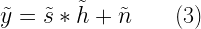
The corresponding complex baseband equivalent (Figure 2(b)) is expressed as
For a given modulation technique, there are two ways to implement the simulation model: passband model and equivalent baseband model. The passband model is also called waveform level simulation model. The waveform level simulation techniques, described in this chapter, are used to represent the physical interactions of the transmitted signal with the channel. In the waveform level simulations, the transmitted signal, the noise and received signal are all represented by samples of waveforms.
Typically, a waveform level simulation uses many samples per symbol. For the computation of error rate performance of various digital modulation techniques, the value of the symbol at the symbol-sampling time instant is all the more important than the look of the entire waveform. In such a case, the detailed waveform level simulation is not required, instead equivalent baseband discrete-time model, described in chapter 3 can be used. Discrete-time equivalent channel model requires only one sample per symbol, hence it consumes less memory and yields results in a very short span of time.
In any communication system, the transmitter operates by modulating the information bearing baseband waveform on to a sinusoidal RF carrier resulting in a passband signal. The carrier frequency, chosen for transmission, varies for different applications. For example, FM radio uses carrier frequency range, whereas for indoor wireless networks the center frequency of transmission is . Hence, the carrier frequency is not the component that contains the information, rather it is the baseband signal that contains the information that is being conveyed.
Actual RF transmission begins by converting the baseband signals to passband signals by the process of up-conversion. Similarly, the passband signals are down-converted to baseband at the receiver, before actual demodulation could begin. Based on this context, two basic types of behavioral models exist for simulation of communication systems – passband models and its baseband equivalent. In the passband model, every cycle of the RF carrier is simulated in detail and the power spectrum will be concentrated near the carrier frequency . Hence, passband models consume more memory, as every point in the RF carrier needs to be stored in computer memory for simulation.
On the other hand, the signals in baseband models are centered near zero frequency. In baseband equivalent models, the RF carrier is suppressed and therefore the number of samples required for simulation is greatly reduced. Furthermore, if the behavior of the system is well understood, the baseband model can be further simplified and the system can be implemented entirely based on the samples at symbol-sampling time instants.
Quadrature Phase Shift Keying (QPSK) is a form of phase modulation technique, in which two information bits (combined as one symbol) are modulated at once, selecting one of the four possible carrier phase shift states.
Figure 1: Waveform simulation model for QPSK modulation
The QPSK signal within a symbol duration \(T_{sym}\) is defined as
\[s(t) = A \cdot cos \left[2 \pi f_c t + \theta_n \right], \quad \quad 0 \leq t \leq T_{sym},\; n=1,2,3,4 \quad \quad (1) \]
Therefore, the four possible initial signal phases are \(\pi/4, 3 \pi/4, 5 \pi/4\) and \(7 \pi/4\) radians. Equation (1) can be re-written as
\[\begin{align} s(t) &= A \cdot cos \theta_n \cdot cos \left( 2 \pi f_c t\right) – A \cdot sin \theta_n \cdot sin \left( 2 \pi f_c t\right) \\ &= s_{ni} \phi_i(t) + s_{nq} \phi_q(t) \quad\quad \quad \quad \quad\quad \quad \quad \quad\quad \quad \quad \quad\quad \quad \quad (3) \end{align} \]
The above expression indicates the use of two orthonormal basis functions: \( \left\langle \phi_i(t),\phi_q(t)\right\rangle\) together with the inphase and quadrature signaling points: \( \left\langle s_{ni}, s_{nq}\right\rangle\). Therefore, on a two dimensional co-ordinate system with the axes set to \( \phi_i(t)\) and \(\phi_q(t)\), the QPSK signal is represented by four constellation points dictated by the vectors \(\left\langle s_{ni}, s_{nq}\right\rangle\) with \( n=1,2,3,4\).
The QPSK transmitter, shown in Figure 1, is implemented as a matlab function qpsk_mod. In this implementation, a splitter separates the odd and even bits from the generated information bits. Each stream of odd bits (quadrature arm) and even bits (in-phase arm) are converted to NRZ format in a parallel manner.
function [s,t,I,Q] = qpsk_mod(a,fc,OF)
%Modulate an incoming binary stream using conventional QPSK
%a - input binary data stream (0's and 1's) to modulate
%fc - carrier frequency in Hertz
%OF - oversampling factor (multiples of fc) - at least 4 is better
%s - QPSK modulated signal with carrier
%t - time base for the carrier modulated signal
%I - baseband I channel waveform (no carrier)
%Q - baseband Q channel waveform (no carrier)
L = 2*OF;%samples in each symbol (QPSK has 2 bits in each symbol)
ak = 2*a-1; %NRZ encoding 0-> -1, 1->+1
I = ak(1:2:end);Q = ak(2:2:end);%even and odd bit streams
I=repmat(I,1,L).'; Q=repmat(Q,1,L).';%even/odd streams at 1/2Tb baud
I = I(:).'; Q = Q(:).'; %serialize
fs = OF*fc; %sampling frequency
t=0:1/fs:(length(I)-1)/fs; %time base
iChannel = I.*cos(2*pi*fc*t);qChannel = -Q.*sin(2*pi*fc*t);
s = iChannel + qChannel; %QPSK modulated baseband signal
The timing diagram for BPSK and QPSK modulation is shown in Figure 2. For BPSK modulation the symbol duration for each bit is same as bit duration, but for QPSK the symbol duration is twice the bit duration: \(T_{sym}=2T_b\). Therefore, if the QPSK symbols were transmitted at same rate as BPSK, it is clear that QPSK sends twice as much data as BPSK does. After oversampling and pulse shaping, it is intuitively clear that the signal on the I-arm and Q-arm are BPSK signals with symbol duration \(2T_b\). The signal on the in-phase arm is then multiplied by \(cos (2 \pi f_c t)\) and the signal on the quadrature arm is multiplied by \(-sin (2 \pi f_c t)\). QPSK modulated signal is obtained by adding the signal from both in-phase and quadrature arms.
Note: The oversampling rate for the simulation is chosen as \(L=2 f_s/f_c\), where \(f_c\) is the given carrier frequency and \(f_s\) is the sampling frequency satisfying Nyquist sampling theorem with respect to the carrier frequency (\(f_s \geq f_c\)). This configuration gives integral number of carrier cycles for one symbol duration.
Figure 2: Timing diagram for BPSK and QPSK modulations
The receiver
Due to its special relationship with BPSK, the QPSK receiver takes the simplest form as shown in Figure 3. In this implementation, the I-channel and Q-channel signals are individually demodulated in the same way as that of BPSK demodulation. After demodulation, the I-channel bits and Q-channel sequences are combined into a single sequence. The function qpsk_demod implements a QPSK demodulator as per Figure 3.
Read more about QPSK, implementation of their modulator and demodulator, performance simulation in these books:
Figure 3: Waveform simulation model for QPSK demodulation
Performance simulation over AWGN
The complete waveform simulation for the aforementioned QPSK modulation and demodulation is given next. The simulation involves, generating random message bits, modulating them using QPSK modulation, addition of AWGN channel noise corresponding to the given signal-to-noise ratio and demodulating the noisy signal using a coherent QPSK receiver. The waveforms at the various stages of the modulator are shown in the Figure 4.
Figure 4: Simulated QPSK waveforms at the transmitter side
The performance simulation for the QPSK transmitter-receiver combination was also coded in the code given above and the resulting bit-error rate performance curve will be same as that of conventional BPSK. A QPSK signal essentially combines two orthogonally modulated BPSK signals. Therefore, the resulting performance curves for QPSK – \(E_b/N_0\) Vs. bits-in-error – will be same as that of conventional BPSK.
QPSK variants
QPSK modulation has several variants, three such flavors among them are: Offset QPSK, π/4-QPSK and π/4-DQPSK.
Offset-QPSK
Offset-QPSK is essentially same as QPSK, except that the orthogonal carrier signals on the I-channel and the Q-channel are staggered (one of them is delayed in time). In OQPSK, the orthogonal components cannot change states at the same time, this is because the components change state only at the middle of the symbol periods (due to the half symbol offset in the Q-channel). This eliminates 180° phase shifts all together and the phase changes are limited to 0° or 90° every bit period.
Elimination of 180° phase shifts in OQPSK offers many advantages over QPSK. Unlike QPSK, the spectrum of OQPSK remains unchanged when band-limited [1]. Additionally, OQPSK performs better than QPSK when subjected to phase jitters [2]. Further improvements to OQPSK can be obtained if the phase transitions are avoided altogether – as evident from continuous modulation schemes like Minimum Shift Keying (MSK) technique.
π/4-QPSK and π/4-DQPSK
In π/4-QPSK, the signaling points of the modulated signals are chosen from two QPSK constellations that are just shifted π/4 radians (45°) with respect to each other. Switching between the two constellations every successive bit ensures that the phase changes are confined to odd multiples of 45°. Therefore, phase transitions of 90° and 180° are eliminated.
π/4-QPSK preserves the constant envelope property better than QPSK and OQPSK. Unlike QPSK and OQPSK schemes, π/4-QPSK can be differentially encoded, therefore enabling the use of both coherent and non-coherent demodulation techniques. Choice of non-coherent demodulation results in simpler receiver design. Differentially encoded π/4-QPSK is referred as π/4-DQPSK.
Read more about QPSK and its variants, implementation of their modulator and demodulator, performance simulation in these books:
Key focus: Compare Performance and spectral efficiency of bandwidth-efficient digital modulation techniques (BPSK,QPSK and QAM) on their theoretical BER over AWGN.
Let’s take up some bandwidth-efficient linear digital modulation techniques (BPSK,QPSK and QAM) and compare its performance based on their theoretical BER over AWGN. (Readers are encouraged to read previous article on Shannon’s theorem and channel capacity).
Table 1 summarizes the theoretical BER (given SNR per bit ration – Eb/N0) for various linear modulations. Note that the Eb/N0 values used in that table are in linear scale [to convert Eb/N0 in dB to linear scale – use Eb/N0(linear) = 10^(Eb/N0(dB)/10) ]. A small script written in Matlab (given below) gives the following output.
Figure 1: Eb/N0 Vs. BER for various digital modulations over AWGN channel
Table 1: Theoretical BER over AWGN for various linear digital modulation techniques
The following table is obtained by extracting the values of Eb/N0 to achieve BER=10-6 from Figure-1. (Table data sorted with increasing values of Eb/N0).
Table 2: Capacity of various modulations their efficiency and channel bandwidth
where,
is the bandwidth efficiency for linear modulation with M point constellation, meaning that ηBbits can be stuffed in one symbol with Rb bits/sec data rate for a given minimum bandwidth.
is the minimum bandwidth needed for information rate of Rb bits/second. If a pulse shaping technique like raised cosine pulse [with roll off factor (a)] is used then Bmin becomes
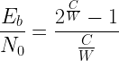
Next the data in table 2 is plotted with Eb/N0 on the x-axis and ηon the y-axis (see figure 2) along with the well known Shannon’s Capacity equation over AWGN given by,
which can be represented as (refer [1])
Figure 2: Spectral efficiency vs Eb/N0 for various modulations at Pb=10-6
Rate this article: Note: There is a rating embedded within this post, please visit this post to rate it.
Matlab Code
EbN0dB=-4:1:24;
EbN0lin=10.^(EbN0dB/10);
colors={'b-*','g-o','r-h','c-s','m-d','y-*','k-p','b-->','g:<','r-.d'};
index=1;

%BPSK
BPSK = 0.5*erfc(sqrt(EbN0lin));
plotHandle=plot(EbN0dB,log10(BPSK),char(colors(index)));
set(plotHandle,'LineWidth',1.5);
hold on;

index=index+1;

%M-PSK
m=2:1:5;
M=2.^m;
for i=M,
    k=log2(i);
    berErr = 1/k*erfc(sqrt(EbN0lin*k)*sin(pi/i));
    plotHandle=plot(EbN0dB,log10(berErr),char(colors(index)));
    set(plotHandle,'LineWidth',1.5);
    index=index+1;
end

%Binary DPSK
Pb = 0.5*exp(-EbN0lin);
plotHandle = plot(EbN0dB,log10(Pb),char(colors(index)));
set(plotHandle,'LineWidth',1.5);
index=index+1;

%Differential QPSK
a=sqrt(2*EbN0lin*(1-sqrt(1/2)));
b=sqrt(2*EbN0lin*(1+sqrt(1/2)));
Pb = marcumq(a,b,1)-1/2.*besseli(0,a.*b).*exp(-1/2*(a.^2+b.^2));
plotHandle = plot(EbN0dB,log10(Pb),char(colors(index)));
set(plotHandle,'LineWidth',1.5);
index=index+1;

%M-QAM
m=2:2:6;
M=2.^m;

for i=M,
    k=log2(i);
    berErr = 2/k*(1-1/sqrt(i))*erfc(sqrt(3*EbN0lin*k/(2*(i-1))));
    plotHandle=plot(EbN0dB,log10(berErr),char(colors(index)));
    set(plotHandle,'LineWidth',1.5);
    index=index+1;
end

legend('BPSK','QPSK','8-PSK','16-PSK','32-PSK','D-BPSK','D-QPSK','4-QAM','16-QAM','64-QAM');
axis([-4 24 -8 0]);
set(gca,'XTick',-4:2:24); %re-name axis accordingly
ylabel('Probability of BER Error - log10(Pb)');
xlabel('Eb/N0 (dB)');
title('Probability of BER Error log10(Pb) Vs Eb/N0');
grid on;
BPSK stands for Binary Phase Shift Keying. It is a type of modulation used in digital communication systems to transmit binary data over a communication channel.
In BPSK, the carrier signal is modulated by changing its phase by 180 degrees for each binary symbol. Specifically, a binary 0 is represented by a phase shift of 180 degrees, while a binary 1 is represented by no phase shift.
BPSK is a straightforward and effective modulation method and is frequently utilized in applications where the communication channel is susceptible to noise and interference. It is also utilized in different wireless communication systems like Wi-Fi, Bluetooth, and satellite communication.
Implementation details
Binary Phase Shift Keying (BPSK) is a two phase modulation scheme, where the 0’s and 1’s in a binary message are represented by two different phase states in the carrier signal: \(\theta=0^{\circ}\) for binary 1 and \(\theta=180^{\circ}\) for binary 0.
In digital modulation techniques, a set of basis functions are chosen for a particular modulation scheme. Generally, the basis functions are orthogonal to each other. Basis functions can be derived using Gram Schmidt orthogonalizationprocedure [1]. Once the basis functions are chosen, any vector in the signal space can be represented as a linear combination of them. In BPSK, only one sinusoid is taken as the basis function. Modulation is achieved by varying the phase of the sinusoid depending on the message bits. Therefore, within a bit duration \(T_b\), the two different phase states of the carrier signal are represented as,
\begin{align*}
s_1(t) &= A_c\; cos\left(2 \pi f_c t \right), & 0 \leq t \leq T_b \quad \text{for binary 1}\\
s_0(t) &= A_c\; cos\left(2 \pi f_c t + \pi \right), & 0 \leq t \leq T_b \quad \text{for binary 0}
\end{align*}
where, \(A_c\) is the amplitude of the sinusoidal signal, \(f_c\) is the carrier frequency \(Hz\), \(t\) being the instantaneous time in seconds, \(T_b\) is the bit period in seconds. The signal \(s_0(t)\) stands for the carrier signal when information bit \(a_k=0\) was transmitted and the signal \(s_1(t)\) denotes the carrier signal when information bit \(a_k=1\) was transmitted.
The constellation diagram for BPSK (Figure 3 below) will show two constellation points, lying entirely on the x axis (inphase). It has no projection on the y axis (quadrature). This means that the BPSK modulated signal will have an in-phase component but no quadrature component. This is because it has only one basis function. It can be noted that the carrier phases are \(180^{\circ}\) apart and it has constant envelope. The carrier’s phase contains all the information that is being transmitted.
BPSK transmitter
A BPSK transmitter, shown in Figure 1, is implemented by coding the message bits using NRZ coding (\(1\) represented by positive voltage and \(0\) represented by negative voltage) and multiplying the output by a reference oscillator running at carrier frequency \(f_c\).
Figure 1: BPSK transmitter
The following function (bpsk_mod) implements a baseband BPSK transmitter according to Figure 1. The output of the function is in baseband and it can optionally be multiplied with the carrier frequency outside the function. In order to get nice continuous curves, the oversampling factor (\(L\)) in the simulation should be appropriately chosen. If a carrier signal is used, it is convenient to choose the oversampling factor as the ratio of sampling frequency (\(f_s\)) and the carrier frequency (\(f_c\)). The chosen sampling frequency must satisfy the Nyquist sampling theorem with respect to carrier frequency. For baseband waveform simulation, the oversampling factor can simply be chosen as the ratio of bit period (\(T_b\)) to the chosen sampling period (\(T_s\)), where the sampling period is sufficiently smaller than the bit period.
function [s_bb,t] = bpsk_mod(ak,L)
%Function to modulate an incoming binary stream using BPSK(baseband)
%ak - input binary data stream (0's and 1's) to modulate
%L - oversampling factor (Tb/Ts)
%s_bb - BPSK modulated signal(baseband)
%t - generated time base for the modulated signal
N = length(ak); %number of symbols
a = 2*ak-1; %BPSK modulation
ai=repmat(a,1,L).'; %bit stream at Tb baud with rect pulse shape
ai = ai(:).';%serialize
t=0:N*L-1; %time base
s_bb = ai;%BPSK modulated baseband signal
BPSK receiver
A correlation type coherent detector, shown in Figure 2, is used for receiver implementation. In coherent detection technique, the knowledge of the carrier frequency and phase must be known to the receiver. This can be achieved by using a Costas loop or a Phase Lock Loop (PLL) at the receiver. For simulation purposes, we simply assume that the carrier phase recovery was done and therefore we directly use the generated reference frequency at the receiver – \(cos( 2 \pi f_c t)\).
Figure 2: Coherent detection of BPSK (correlation type)
In the coherent receiver, the received signal is multiplied by a reference frequency signal from the carrier recovery blocks like PLL or Costas loop. Here, it is assumed that the PLL/Costas loop is present and the output is completely synchronized. The multiplied output is integrated over one bit period using an integrator. A threshold detector makes a decision on each integrated bit based on a threshold. Since, NRZ signaling format was used in the transmitter, the threshold for the detector would be set to \(0\). The function bpsk_demod, implements a baseband BPSK receiver according to Figure 2. To use this function in waveform simulation, first, the received waveform has to be downconverted to baseband, and then the function may be called.
function [ak_cap] = bpsk_demod(r_bb,L)
%Function to demodulate an BPSK(baseband) signal
%r_bb - received signal at the receiver front end (baseband)
%N - number of symbols transmitted
%L - oversampling factor (Tsym/Ts)
%ak_cap - detected binary stream
x=real(r_bb); %I arm
x = conv(x,ones(1,L));%integrate for L (Tb) duration
x = x(L:L:end);%I arm - sample at every L
ak_cap = (x > 0).'; %threshold detector
End-to-end simulation
The complete waveform simulation for the end-to-end transmission of information using BPSK modulation is given next. The simulation involves: generating random message bits, modulating them using BPSK modulation, addition of AWGN noise according to the chosen signal-to-noise ratio and demodulating the noisy signal using a coherent receiver. The topic of adding AWGN noise according to the chosen signal-to-noise ratio is discussed in section 4.1 in chapter 4. The resulting waveform plots are shown in the Figure 2.3. The performance simulation for the BPSK transmitter/receiver combination is also coded in the program shown next (see chapter 4 for more details on theoretical error rates).
The resulting performance curves will be same as the ones obtained using the complex baseband equivalent simulation technique in Figure 4.4 of chapter 4.
File 3: bpsk_wfm_sim.m: Waveform simulation for BPSK modulation and demodulation
Figure 3: (a) Baseband BPSK signal,(b) transmitted BPSK signal – with carrier, (c) constellation at transmitter and (d) received signal with AWGN noise
This website uses cookies to improve your experience while you navigate through the website. Out of these, the cookies that are categorized as necessary are stored on your browser as they are essential for the working of basic functionalities of the website. We also use third-party cookies that help us analyze and understand how you use this website. These cookies will be stored in your browser only with your consent. You also have the option to opt-out of these cookies. But opting out of some of these cookies may affect your browsing experience.
Necessary cookies are absolutely essential for the website to function properly. These cookies ensure basic functionalities and security features of the website, anonymously.
Cookie
Duration
Description
cookielawinfo-checbox-analytics
11 months
This cookie is set by GDPR Cookie Consent plugin. The cookie is used to store the user consent for the cookies in the category "Analytics".
cookielawinfo-checbox-analytics
11 months
This cookie is set by GDPR Cookie Consent plugin. The cookie is used to store the user consent for the cookies in the category "Analytics".
cookielawinfo-checbox-functional
11 months
The cookie is set by GDPR cookie consent to record the user consent for the cookies in the category "Functional".
cookielawinfo-checbox-functional
11 months
The cookie is set by GDPR cookie consent to record the user consent for the cookies in the category "Functional".
cookielawinfo-checbox-others
11 months
This cookie is set by GDPR Cookie Consent plugin. The cookie is used to store the user consent for the cookies in the category "Other.
cookielawinfo-checbox-others
11 months
This cookie is set by GDPR Cookie Consent plugin. The cookie is used to store the user consent for the cookies in the category "Other.
cookielawinfo-checkbox-necessary
11 months
This cookie is set by GDPR Cookie Consent plugin. The cookies is used to store the user consent for the cookies in the category "Necessary".
cookielawinfo-checkbox-performance
11 months
This cookie is set by GDPR Cookie Consent plugin. The cookie is used to store the user consent for the cookies in the category "Performance".
viewed_cookie_policy
11 months
The cookie is set by the GDPR Cookie Consent plugin and is used to store whether or not user has consented to the use of cookies. It does not store any personal data.
Functional cookies help to perform certain functionalities like sharing the content of the website on social media platforms, collect feedbacks, and other third-party features.
Performance cookies are used to understand and analyze the key performance indexes of the website which helps in delivering a better user experience for the visitors.
Analytical cookies are used to understand how visitors interact with the website. These cookies help provide information on metrics the number of visitors, bounce rate, traffic source, etc.


![a[k]](https://s0.wp.com/latex.php?latex=a%5Bk%5D&bg=ffffff&fg=000&s=0&c=20201002)

![b[k] = b[k-1] \oplus a[k] \;\;\;\;\;\; (modulo-2) \;\;\;\;\;\; (1)](https://s0.wp.com/latex.php?latex=b%5Bk%5D+%3D+b%5Bk-1%5D+%5Coplus+a%5Bk%5D+%5C%3B%5C%3B%5C%3B%5C%3B%5C%3B%5C%3B+%28modulo-2%29+%5C%3B%5C%3B%5C%3B%5C%3B%5C%3B%5C%3B+%281%29+&bg=ffffff&fg=000&s=2&c=20201002)

![a[k] = b[k] \oplus b[k-1] \;\;\;\;\;\; (modulo-2) \;\;\;\;\;\; (2)](https://s0.wp.com/latex.php?latex=a%5Bk%5D+%3D+b%5Bk%5D+%5Coplus+b%5Bk-1%5D%C2%A0+%5C%3B%5C%3B%5C%3B%5C%3B%5C%3B%5C%3B+%28modulo-2%29+%5C%3B%5C%3B%5C%3B%5C%3B%5C%3B%5C%3B+%282%29+&bg=ffffff&fg=000&s=2&c=20201002)


![P_b = erfc \left(\sqrt{\frac{E_b}{N_0}} \right) \left[ 1-\frac{1}{2} erfc \left( \sqrt{\frac{E_b}{N_0}} \right) \right] \;\; (3)](https://s0.wp.com/latex.php?latex=P_b+%3D+erfc+%5Cleft%28%5Csqrt%7B%5Cfrac%7BE_b%7D%7BN_0%7D%7D+%5Cright%29+%5Cleft%5B+1-%5Cfrac%7B1%7D%7B2%7D+erfc+%5Cleft%28+%5Csqrt%7B%5Cfrac%7BE_b%7D%7BN_0%7D%7D+%5Cright%29+%5Cright%5D+%5C%3B%5C%3B+%283%29+&bg=ffffff&fg=000&s=2&c=20201002)


![\tilde{s}(t) = a(t) cos \left[ 2 \pi f_c t + \phi(t) \right] = s_I(t) cos(2 \pi f_c t) - s_Q(t) sin(2 \pi f_c t) \quad (1)](https://s0.wp.com/latex.php?latex=%5Ctilde%7Bs%7D%28t%29+%3D+a%28t%29+cos+%5Cleft%5B+2+%5Cpi+f_c+t+%2B+%5Cphi%28t%29+%5Cright%5D+%3D+s_I%28t%29+cos%282+%5Cpi+f_c+t%29+-+s_Q%28t%29+sin%282+%5Cpi+f_c+t%29+%5Cquad+%281%29+&bg=ffffff&fg=000&s=2&c=20201002)