Note: There is a rating embedded within this post, please visit this post to rate it.
As a pre-requisite, check out the previous article on the logic behind deriving the maximum likelihood estimator for a given PDF.
Let X=(x1,x2,…, xN) are the samples taken from Gaussian distribution given by
Calculating the Likelihood
The log likelihood is given by,
Differentiating and equating to zero to find the maxim (otherwise equating the score to zero)
Thus the mean of the samples gives the MLE of the parameter .
Note: There is a rating embedded within this post, please visit this post to rate it.
As a pre-requisite, check out the previous article on the logic behind deriving the maximum likelihood estimator for a given PDF.
Let X=(x1,x2,…, xN) are the samples taken from Exponential distribution given by
Calculating the Likelihood
The log likelihood is given by,
Differentiating and equating to zero to find the maxim (otherwise equating the score to zero)
Thus the inverse of mean of the samples gives the MLE of the parameter .
Note: There is a rating embedded within this post, please visit this post to rate it.
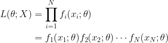
Suppose X=(x1,x2,…, xN) are the samples taken from a random distribution whose PDF is parameterized by the parameter . If the PDF of the underlying parameter satisfies some regularity condition (if the log of the PDF is differentiable) then the likelihood function is given by
Here is the PDF of the underlying distribution.
Hereafter we will denote as .
The maximum likelihood estimate of the unknown parameter can be found by selecting the say some for which the likelihood function attains maximum. We usually use log of the likelihood function to simplify multiplications into additions. So restating this, the maximum likelihood estimate of the unknown parameter can be found by selecting the say some for which the log likelihood function attains maximum.
In differential geometry, the maximum of a function f(x) is found by taking the first derivative of the function and equating it to zero. Similarly, the maximum likelihood estimate of a parameter – is found by partially differentiating the likelihood function or the log likelihood function and equating it to zero.
The first partial derivative of log likelihood function with respect to is also called score. The variance of the score (partial derivative of score with respect to ) is known as Fisher Information.
Calculating MLE for Poisson distribution:
Let X=(x1,x2,…, xN) are the samples taken from Poisson distribution given by
Calculating the Likelihood
The log likelihood is given by,
Differentiating and equating to zero to find the maxim (otherwise equating the score to zero)
Thus the mean of the samples gives the MLE of the parameter .
To be updated soon
For the derivation of other PDFs see the following links
Theoretical derivation of Maximum Likelihood Estimator for Exponential PDF
Theoretical derivation of Maximum Likelihood Estimator for Gaussian PDF
Key focus: Understand maximum likelihood estimation (MLE) using hands-on example. Know the importance of log likelihood function and its use in estimation problems.
Likelihood Function:
Suppose X=(x1,x2,…, xN) are the samples taken from a random distribution whose PDF is parameterized by the parameter θ. The likelihood function is given by
Here fN(xN;θ) is the PDF of the underlying distribution.
The above equation differs significantly from the joint probability calculation that in joint probability calculation, θ is considered a random variable. In the above equation, the parameter θ is the parameter to be estimated.
Example:
Consider the DC estimation problem presented in the previous article where a transmitter transmits continuous stream of data samples representing a constant value – A. The data samples sent via a communication channel gets added with White Gaussian Noise – w[n] (with μ=0 and σ2=1 ). The receiver receives the samples and its goal is to estimate the actual DC component – A in the presence of noise.
Figure 1: The problem of DC estimation
Likelihood as an Estimation Metric:
Let’s use the likelihood function as estimation metric. The estimation of A depends on the PDF of the underlying noise-w[n]. The estimation accuracy depends on the variance of the noise. More the variance less is the accuracy of estimation and vice versa.
Let’s fix A=1.3 and generate 10 samples from the above model (Use the Matlab script given below to test this. You may get different set of numbers). Now we pretend that we do not know anything about the model and all we want to do is to estimate the DC component (Parameter to be estimated θ=A) from the observed samples:
Assuming a variance of 1 for the underlying PDF, we will try a range of values for A from -2.0 to +1.5 in steps of 0.1 and calculate the likelihood function for each value of A.
Matlab script:
% Demonstration of Maximum Likelihood Estimation in Matlab
%   Author: Mathuranathan (https://www.gaussianwaves.com)
%   License : creative commons : Attribution-NonCommercial-ShareAlike 3.0 Unported

A=1.3;
N=10; %Number of Samples to collect
x=A+randn(1,N);

s=1; %Assume standard deviation s=1

rangeA=-2:0.1:5; %Range of values of estimation parameter to test
L=zeros(1,length(rangeA)); %Place holder for likelihoods

for i=1:length(rangeA)
    %Calculate Likelihoods for each parameter value in the range
    L(i) = exp(-sum((x-rangeA(i)).^2)/(2*s^2));  %Neglect the constant term (1/(sqrt(2*pi)*sigma))^N as it will pull %down the likelihood value to zero for increasing value of N
end

[maxL,index]=max(L); %Select the parameter value with Maximum Likelihood
display('Maximum Likelihood of A');
display(rangeA(index));

%Plotting Commands
plot(rangeA,L);hold on;
stem(rangeA(index),L(index),'r'); %Point the Maximum Likelihood Estimate
displayText=['\leftarrow Likelihood of A=' num2str(rangeA(index))];
title('Maximum Likelihood Estimation of unknown Parameter A');
xlabel('\leftarrow A');
ylabel('Likelihood');
text(rangeA(index),L(index)/3,displayText,'HorizontalAlignment','left');

figure(2);
plot(rangeA,log(L));hold on;
YL = ylim;YMIN = YL(1);
plot([rangeA(index) rangeA(index)],[YMIN log(L(index))] ,'r'); %Point the Maximum Likelihood Estimate
title('Log Likelihood Function');
xlabel('\leftarrow A');
ylabel('Log Likelihood');
text([rangeA(index)],YMIN/2,displayText,'HorizontalAlignment','left');
Simulation Result:
For the above mentioned 10 samples of observation, the likelihood function over the range (-2:0.1:1.5) of DC component values is plotted below. The maximum likelihood value happens at A=1.4 as shown in the figure. The estimated value of A is 1.4 since the maximum value of likelihood occurs there.
This estimation technique based on maximum likelihood of a parameter is called Maximum Likelihood Estimation (MLE). The estimation accuracy will increase if the number of samples for observation is increased. Try the simulation with the number of samples N set to 5000 or 10000 and observe the estimated value of A for each run.
Figure 2: Maximum likelihood estimation of unknown parameter A
Log Likelihood Function:
It is often useful to calculate the log likelihood function as it reduces the above mentioned equation to series of additions instead of multiplication of several terms. This is particularly useful when implementing the likelihood metric in digital signal processors. The log likelihood is simply calculated by taking the logarithm of the above mentioned equation. The decision is again based on the maximum likelihood criterion.
Figure 3: Maximum likelihood estimation using log likelihood function
Advantages of Maximum Likelihood Estimation:
* Asymptotically Efficient – meaning that the estimate gets better with more samples * Asymptotically unbiased * Asymptotically consistent * Easier to compute * Estimation without any prior information * The estimates closely agree with the data
Disadvantages of Maximum Likelihood Estimation:
* Since the estimates closely agree with data, it will give noisy estimates for data mixed with noise. * It does not utilize any prior information for the estimation. But in real world scenario, we always have some prior information about the parameter to be estimated. We should always use it to our advantage despite it introducing bias in the estimates.
Rate this article: Note: There is a rating embedded within this post, please visit this post to rate it.
Estimator bias: Systematic deviation from the true value, either consistently overestimating or underestimating the parameter of interest.
Estimator Bias: Biased or Unbiased
Consider a simple communication system model where a transmitter transmits continuous stream of data samples representing a constant value – ‘A’. The data samples sent via a communication channel gets added with White Gaussian Noise – ‘w[n]’ (with mean=0 and variance=1). The receiver receives the samples and its goal is to estimate the actual constant value (we will call it DC component hereafter) transmitted by the transmitter in the presence of noise. This is a classical DC estimation problem.
Since the constant DC component is embedded in noise, we need to come up with an estimator function to estimate the DC component from the received samples. The goal of our estimator function is to estimate the DC component so that the mean of the estimate should be equal to the actual DC value. This is the criteria for ascertaining the unbiased-ness of an estimator.
The following figure captures the difference between a biased estimator and an unbiased estimator.
Example for understanding estimator bias
Consider that we are presented with a set of N samples of data representing x[n] at the receiver. Let’s us take the signal model that represents the received data samples :
Consider two estimator models/functions to estimate the DC component from the received samples. We will see which of the two estimator functions gives us unbiased estimate.
\( \begin{align} &= A; if \; A=0 \\ & \neq A; if \; A \neq 0 \end{align} \)
Bias
Unbiased
Biased
Testing the bias of an estimation in Matlab:
To test the bias of the above mentioned estimators in Matlab, the signal model: \(x[n]=A+w[n]\) is taken as a starting point. Here \(A\) is a constant DC value (say for example it takes a value of 1.5) and w[n] is a vector of random noise that follows standard normal distribution with mean=0 and variance=1.
Generate 5000 signal samples \(x[n]\) by setting \(A=1.5\) and adding it with \(w[n]\) generated using Matlab’s “randn” function.
N=5000; %Number of samples for the test
A=1.5 ;%Actual DC value
w = randn(1,N); %Standard Normal Distribution mean=0,variance=1 represents noise
x = A + w ;  %Received signal samples
Implement the above mentioned estimator functions and display their estimated values
estA1 = sum(x)/N;%  Estimated DC component from x[n] using estimator 1
estA2 = sum(x)/(2*N); %  Estimated DC component from x[n] using estimator 2

%Display estimated values
disp([‘Estimator 1: ’ num2str(estA1) ]);
disp([‘Estimator 2: ’ num2str(estA2) ]);
Sample Result :
Estimator 1: 1.5185 % Estimator 1’s result will near exact value of 1.5 as N grows larger
Estimator 2: 0.75923 % Estimator 2’s result is biased as it is far away from the actual DC value
The above result just prints the estimated value. Since the estimated parameter – \(\hat{A}\) is a constant \(E(\hat{A}) = \hat{A}\). In real world scenario, the parameter that is estimated, will be a random variable. In that case you have to print the “expectation” (mean) of the estimated value for comparison.
As discussed in the introduction to estimation theory, the goal of an estimation algorithm is to give an estimate of random variable(s) that is unbiased and has minimum variance. This criteria is reproduced here for reference
In the above equations f0 is the transmitted carrier frequency and is the estimated frequency based on a set of observed data (See previous article).
Existence of minimum-variance unbiased estimator (MVUE):
The estimator described above is called minimum-variance unbiased estimator (MVUE) since, the estimates are unbiased as well as they have minimum variance. Sometimes there may not exist any MVUE for a given scenario or set of data. This can happen in two ways 1) No existence of unbiased estimators 2) Even if we have unbiased estimator, none of them gives uniform minimum variance.
Consider that we have three unbiased estimators g1, g2 and g3 that gives estimates of a deterministic parameter θ. Let the unbiased estimates be , and respectively.
Figure 1 illustrates two scenarios for the existence of an MVUE among the three estimators. In Figure 1a, the third estimator gives uniform minimum variance compared to other two estimators. In Figure 1b, none of the estimator gives minimum variance that is uniform across the entire range of θ.
Figure 1: Illustration of existence of Minimum Variable Unbiased Estimator (MVUE)
2) Use Rao-Blackwell-Lechman-Scheffe (RBLS) Theorem: Find a sufficient statistic and find a function of the sufficient statistic. This function gives the MVUE. This approach is rarely used in practice.
3) Restrict the solution to find linear estimators that are unbiased. This gives Minimum Variance Linear Unbiased Estimator (MVLUE). This method gives MVLUE only if the problem is truly linear.
Rate this article: Note: There is a rating embedded within this post, please visit this post to rate it.
Key focus: Understand the basics of estimation theory with a simple example in communication systems. Know how to assess the performance of an estimator.
A simple estimation problem : DSB-AM receiver
In Double Side Band – Amplitude Modulation (DSB-AM), the desired message is amplitude modulated over a carrier of frequency f0. The following discussion is with reference to the figure 1. In the frequency domain, the spectrum of the message signal, which is a baseband signal, may look like the one shown in (a). After the modulation over a carrier frequency off0, the spectrum of the modulated signal will look like as shown in (b). The modulated signal has spectral components centered at f0 and -f0.
Figure 1: Illustrating estimation of unknowns f and Φ using DSB-AM receiver
The modulated signal is a function of three factors : 1) actual message – m(t) 2) carrier frequency – f0 3) phase uncertainty – Φ0
The modulated signal can be expressed as,
To simplify things, let’s consider that the modulated signal is passed via an ideal channel (no impairments added by the channel, so we can do away with channel equalization and other complex stuffs in the receiver). The modulated signal hits the antenna located at front end of our DSBC receiver. Usually the receiver front end is employed with a band-pass filter and amplifier to put the received signal in the desired band of operation & level, as expected by the receiver. The electronics in the front end receiver adds noise to the incoming signal (modeled as white noise – w(t) ). The signal after the BPF and amplifier combination is expressed as x(t), which is a combination of our desired signal s(t) and the front end noise w(t). Thus x(t) can be expressed as
The signal x(t) is band-pass (centered around the carrier frequency f0). To bring x(t) back to the baseband, a mixer is employed that multiplies x(t) with a tone centered at f0 (generated by a local oscillator). Actually a low pass filter is usually employed after the mixer, for extracting the desired signal at the baseband.
As the receiver has no knowledge about the carrier frequency, there must exist a technique/method to extract this information from the incoming signal x(t) itself. Not only the carrier frequency (f0) but also the phase Φ0 of the carrier need to be known at the receiver for proper demodulation. This leads us to the problem of “estimation”.
Estimation of unknown parameters
In “estimation” problem, we are confronted with estimating one or more unknown parameters based on a sequence of observed data. In our problem, the signal x(t) is the observed data and the parameters that are to be estimated are f0 and Φ0 .
Now, we add an estimation algorithm at the receiver, that takes in the signal x(t) and computes estimates of f0 and Φ0.The estimated values are denoted with a cap on their respective letters.The estimation algorithm can be simply stated as follows
Given , estimate and that are optimal in some sense.
So far, all the notations were expressed in continuous domain. To simplify calculations, let’s state the estimation problem in discrete time domain. In discrete time domain, the samples of observed signal – which is a combination of actual signal and noise is expressed As
The noise samples w[n] is a random variable, that randomizes every time we observe x[n]. Each time when we observe the “observed” samples – x[n] , we think of it as having the same “actual” signal samples – s[n] but with different realizations of the noise samples w[n]. Thus w[n] can be modeled as a Random Variable (RV). Since the underlying noise w[n] is a random variable, the estimates and that result from the estimation are also random variables.
Now the estimation algorithm can be stated as follows:
Given the observed data samples – x[n] = ( x[0], x[1],x[2], … ,x[N-1] ), our goal is to find estimator functions that maps the given data into estimates.
Assessing the performance of the estimation algorithm
Since the estimates and are random variables, they can be described by a probability density function (PDF). The PDF of the estimates depend on following factors :
1. Structure of s[n] 2. Probability model of w[n] 3. Form of estimation function g(x)
For example, the PDF of the estimate may take the following shape,
Figure 2: Probability Density function of estimate – f
The goal of the estimation algorithm is to give an estimate that is unbiased (mean of the estimate is equal to the actual f0) and has minimum variance. This criteria can be expressed as,
Same type of argument will hold for the other estimate :
This website uses cookies to improve your experience while you navigate through the website. Out of these, the cookies that are categorized as necessary are stored on your browser as they are essential for the working of basic functionalities of the website. We also use third-party cookies that help us analyze and understand how you use this website. These cookies will be stored in your browser only with your consent. You also have the option to opt-out of these cookies. But opting out of some of these cookies may affect your browsing experience.
Necessary cookies are absolutely essential for the website to function properly. These cookies ensure basic functionalities and security features of the website, anonymously.
Cookie
Duration
Description
cookielawinfo-checbox-analytics
11 months
This cookie is set by GDPR Cookie Consent plugin. The cookie is used to store the user consent for the cookies in the category "Analytics".
cookielawinfo-checbox-analytics
11 months
This cookie is set by GDPR Cookie Consent plugin. The cookie is used to store the user consent for the cookies in the category "Analytics".
cookielawinfo-checbox-functional
11 months
The cookie is set by GDPR cookie consent to record the user consent for the cookies in the category "Functional".
cookielawinfo-checbox-functional
11 months
The cookie is set by GDPR cookie consent to record the user consent for the cookies in the category "Functional".
cookielawinfo-checbox-others
11 months
This cookie is set by GDPR Cookie Consent plugin. The cookie is used to store the user consent for the cookies in the category "Other.
cookielawinfo-checbox-others
11 months
This cookie is set by GDPR Cookie Consent plugin. The cookie is used to store the user consent for the cookies in the category "Other.
cookielawinfo-checkbox-necessary
11 months
This cookie is set by GDPR Cookie Consent plugin. The cookies is used to store the user consent for the cookies in the category "Necessary".
cookielawinfo-checkbox-performance
11 months
This cookie is set by GDPR Cookie Consent plugin. The cookie is used to store the user consent for the cookies in the category "Performance".
viewed_cookie_policy
11 months
The cookie is set by the GDPR Cookie Consent plugin and is used to store whether or not user has consented to the use of cookies. It does not store any personal data.
Functional cookies help to perform certain functionalities like sharing the content of the website on social media platforms, collect feedbacks, and other third-party features.
Performance cookies are used to understand and analyze the key performance indexes of the website which helps in delivering a better user experience for the visitors.
Analytical cookies are used to understand how visitors interact with the website. These cookies help provide information on metrics the number of visitors, bounce rate, traffic source, etc.


![\sigma^{2}_{\hat{f}_0}= E \left\{ ( \hat{f}_0 - E [ \hat{f}_0 ] )^2 \right\}](https://s0.wp.com/latex.php?latex=%5Csigma%5E%7B2%7D_%7B%5Chat%7Bf%7D_0%7D%3D+E+%5Cleft%5C%7B+%28+%5Chat%7Bf%7D_0+-+E+%5B+%5Chat%7Bf%7D_0+%5D+%29%5E2+%5Cright%5C%7D+&bg=ffffff&fg=000&s=1&c=20201002)


![x[n] = s[n;f_0, \phi_0] + w[n]](https://s0.wp.com/latex.php?latex=x%5Bn%5D+%3D+s%5Bn%3Bf_0%2C+%5Cphi_0%5D+%2B+w%5Bn%5D+&bg=ffffff&fg=000&s=2&c=20201002)

![\hat{f}_{0}=g_{1}(x[0], x[1],x[2],\cdots,x[N-1])=g_{1} \left( \textbf{x} \right)](https://s0.wp.com/latex.php?latex=%5Chat%7Bf%7D_%7B0%7D%3Dg_%7B1%7D%28x%5B0%5D%2C+x%5B1%5D%2Cx%5B2%5D%2C%5Ccdots%2Cx%5BN-1%5D%29%3Dg_%7B1%7D+%5Cleft%28+%5Ctextbf%7Bx%7D+%5Cright%29+&bg=ffffff&fg=000&s=2&c=20201002)

![\hat{\phi}_{0} = g_{2} (x[0], x[1], x[2], \cdots, x[N-1]) = g_{2} \left( \textbf{x} \right)](https://s0.wp.com/latex.php?latex=%5Chat%7B%5Cphi%7D_%7B0%7D+%3D+g_%7B2%7D+%28x%5B0%5D%2C+x%5B1%5D%2C+x%5B2%5D%2C+%5Ccdots%2C+x%5BN-1%5D%29+%3D+g_%7B2%7D+%5Cleft%28+%5Ctextbf%7Bx%7D+%5Cright%29+&bg=ffffff&fg=000&s=2&c=20201002)


![\begin{aligned} E\left\{\hat{f}_0 \right\} &= f_0 \\ \sigma^{2}_{\hat{f}_0} &= E \left\{ \left( \hat{f}_0 - E [ \hat{f}_0] \right)^2 \right\} \quad \text{should be minimum} \end{aligned}](https://s0.wp.com/latex.php?latex=%5Cbegin%7Baligned%7D+E%5Cleft%5C%7B%5Chat%7Bf%7D_0+%5Cright%5C%7D+%26%3D+f_0+%5C%5C+%5Csigma%5E%7B2%7D_%7B%5Chat%7Bf%7D_0%7D+%26%3D+E+%5Cleft%5C%7B+%5Cleft%28+%5Chat%7Bf%7D_0+-+E+%5B+%5Chat%7Bf%7D_0%5D+%5Cright%29%5E2+%5Cright%5C%7D+%5Cquad+%5Ctext%7Bshould+be+minimum%7D+%5Cend%7Baligned%7D+&bg=ffffff&fg=000&s=2&c=20201002)