Linear Models – Least Squares Estimator (LSE)

Key focus: Understand step by step, the least squares estimator for parameter estimation. Hands-on example to fit a curve using least squares estimation

Background:

The various estimation concepts/techniques like Maximum Likelihood Estimation (MLE), Minimum Variance Unbiased Estimation (MVUE), Best Linear Unbiased Estimator (BLUE) – all falling under the umbrella of classical estimation – require assumptions/knowledge on second order statistics (covariance) before the estimation technique can be applied. Linear estimators, discussed here, do not require any statistical model to begin with. It only requires a signal model in linear form.

Linear models are ubiquitously used in various fields for studying the relationship between two or more variables. Linear models include regression analysis models, ANalysis Of VAriance (ANOVA) models, variance component models etc. Here, one variable is considered as a dependent (response) variable which can be expressed as a linear combination of one or more independent (explanatory) variables.

Studying the dependence between variables is fundamental to linear models. For applying the concepts to real application, following procedure is required

  1. Problem identification
  2. Model selection
  3. Statistical performance analysis
  4. Criticism of the model based on statistical analysis
  5. Conclusions and recommendations

Following text seeks to elaborate on linear models when applied to parameter estimation using Ordinary Least Squares (OLS).

Linear Regression Model

A regression model relates a dependent (response) variable y to a set of k independent explanatory variables {x1, x2 ,…, xk} using a function. When the relationship is not exact, an error term e is introduced.

If the function f is not a linear function, the above model is referred as Non-Linear Regression Model. If f is linear, equation (1) is expressed as linear combination of independent variables xk weighted by unknown vector parameters θ = {θ1, θ2,…, θk } that we wish to estimate.

Equation (2) is referred as Linear Regression model. When N such observations are made

where,
yi – response variable
xi – independent variables – known expressed as observed matrix X with rank k
θi – set of parameters to be estimated
e – disturbances/measurement errors – modeled as noise vector with PDF N(0, σ2 I)

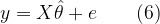
It is convenient to express all the variables in matrix form when N observations are made.

Denoting equation (3) using (4),

Except for X which is a matrix, all other variables are column/row vectors.

Ordinary Least Squares Estimation (OLS)

In OLS – all errors are considered equal as opposed to Weighted Least Squares where some errors are considered significant than others.

If is a k ⨉ 1 vector of estimates of θ, then the estimated model can be written as

Thus the error vector e can be computed from the observed data matrix y and the estimated as

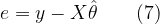
Here, the errors are assumed to be following multivariate normal distribution with zero mean and standard deviation σ2.

To determine the least squares estimator, we write the sum of squares of the residuals (as a function of ) as

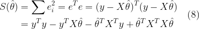
The least squares estimator is obtained by minimizing . In order to get the estimate that gives the least square error, differentiate with respect to and equate to zero.

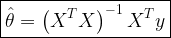
Thus, the least squared estimate of θ is given by

where the operator T denotes Hermitian Transpose (conjugate transpose).

Summary of computations

  1. Step 1: Choice of variables. Choose the variable to be explained (y) and the explanatory variables { x1, x2 ,…, xk } where x1 is often considered a constant (optional) that always takes the value 1 – this is to incorporate a DC component in the model.
  2. Step 2: Collect data. Collect n observations of y and for a set of known values of { x1, x2 ,…, xk }. Example: { x1, x2 ,…, xk } is the pilot data in OFDM using which we would like to estimate the channel impulse response θ and y is the received vector of samples. Store the observed data y in an – n⨉1 vector and the data on the explanatory variables in the n⨉k matrix X.
  3. Step 3: Compute the estimates. Compute the least squares estimates by the formula

The superscript T indicates Hermitian Transpose (conjugate transpose) operation.

Key Points

  • We do not need a probabilistic assumption but only a deterministic signal model.
  • It has a broader range of applications.
  • Least squares is unbiased.
  • Estimating the disturbance variance (k variables to estimate and n observations are available).
  • To keep the variance low, the number of observations must be greater than the number of variables to estimate.
  • The observation matrix X should have maximum rank – this leads to independent rows and columns which always happens with real data. This will make sure (XTX) is invertible.
  • Least Squares Estimator can be used in block processing mode with overlapping segments – similar to Welch’s method of PSD estimation.
  • Useful in time-frequency analysis.
  • Adaptive filters are utilized for non-stationary applications.

LSE applied to curve fitting

Matlab snippet for implementing Least Estimate to fit a curve is given below.

x = -5:.1:5; % set of x- values - known explanatory variables
y = 5.3 + 1.2* x; % Straight line without noise
e=randn(size(y));
y = y + e; % adding random noise to get observed variable - 
%Linear model - Y=Xa+e where a - parameters to be estimated

X = [ ones(length(x),1) x']; %first column treated aas all ones since x_1=1
y = y'; %column vector for proper dimension during multiplication
a = inv(X'*X)*X'*y  % Least Squares Estimator - equivalent code X\y
h=plot ( x , y , 'o'); %original data
hold on;
plot( x , a(1)+ a(2)*x , 'r-' ); %Fitted line
legend('observed samples',['y=' num2str(a(1)) '+' num2str(a(2)) 'x']) 
title('Least Squares Estimate for Curve Fitting');
xlabel('X values');
ylabel('Y values');

Simulation Results

Least Squares Estimate for Curve Fitting Matlab
Figure 1: Least Squares Estimate for Curve Fitting

Rate this article: Note: There is a rating embedded within this post, please visit this post to rate it.

Related topics:

[1]An Introduction to Estimation Theory
[2]Bias of an Estimator
[3]Minimum Variance Unbiased Estimators (MVUE)
[4]Maximum Likelihood Estimation
[5]Maximum Likelihood Decoding
[6]Probability and Random Process
[7]Likelihood Function and Maximum Likelihood Estimation (MLE)
[8]Score, Fisher Information and Estimator Sensitivity
[9]Introduction to Cramer Rao Lower Bound (CRLB)
[10]Cramer Rao Lower Bound for Scalar Parameter Estimation
[11]Applying Cramer Rao Lower Bound (CRLB) to find a Minimum Variance Unbiased Estimator (MVUE)
[12]Efficient Estimators and CRLB
[13]Cramer Rao Lower Bound for Phase Estimation
[14]Normalized CRLB - an alternate form of CRLB and its relation to estimator sensitivity
[15]Cramer Rao Lower Bound (CRLB) for Vector Parameter Estimation
[16]The Mean Square Error – Why do we use it for estimation problems
[17]How to estimate unknown parameters using Ordinary Least Squares (OLS)
[18]Essential Preliminary Matrix Algebra for Signal Processing
[19]Why Cholesky Decomposition ? A sample case:
[20]Tests for Positive Definiteness of a Matrix
[21]Solving a Triangular Matrix using Forward & Backward Substitution
[22]Cholesky Factorization - Matlab and Python
[23]LTI system models for random signals – AR, MA and ARMA models
[24]Comparing AR and ARMA model - minimization of squared error
[25]Yule Walker Estimation
[26]AutoCorrelation (Correlogram) and persistence – Time series analysis
[27]Linear Models - Least Squares Estimator (LSE)
[28]Best Linear Unbiased Estimator (BLUE)

Books by the author


Wireless Communication Systems in Matlab
Second Edition(PDF)

Note: There is a rating embedded within this post, please visit this post to rate it.
Checkout Added to cart

Digital Modulations using Python
(PDF ebook)

Note: There is a rating embedded within this post, please visit this post to rate it.
Checkout Added to cart

Digital Modulations using Matlab
(PDF ebook)

Note: There is a rating embedded within this post, please visit this post to rate it.
Checkout Added to cart
Hand-picked Best books on Communication Engineering
Best books on Signal Processing

Estimator Bias

Estimator bias: Systematic deviation from the true value, either consistently overestimating or underestimating the parameter of interest.

Estimator Bias: Biased or Unbiased

Consider a simple communication system model where a transmitter transmits continuous stream of data samples representing a constant value – ‘A’. The data samples sent via a communication channel gets added with White Gaussian Noise – ‘w[n]’ (with mean=0 and variance=1). The receiver receives the samples and its goal is to estimate the actual constant value (we will call it DC component hereafter) transmitted by the transmitter in the presence of noise. This is a classical DC estimation problem.

Since the constant DC component is embedded in noise, we need to come up with an estimator function to estimate the DC component from the received samples. The goal of our estimator function is to estimate the DC component so that the mean of the estimate should be equal to the actual DC value. This is the criteria for ascertaining the unbiased-ness of an estimator.

The following figure captures the difference between a biased estimator and an unbiased estimator.

Example for understanding estimator bias

Consider that we are presented with a set of N samples of data representing x[n] at the receiver. Let’s us take the signal model that represents the received data samples :

\[\begin{align} Signal\; Model: x[n] = A + w[n] ; & \quad n = 0,1, \cdots, N-1 \\ & \quad w[n] \sim \mathcal{N}(0,1) \end{align}\]

Consider two estimator models/functions to estimate the DC component from the received samples. We will see which of the two estimator functions gives us unbiased estimate.

\[\begin{align} \text{Estimator 1}: \hat{A} &= \frac{1}{N} \sum_{n=0}^{N-1} x[n] \\ \text{Estimator 2}: \hat{A} &= \frac{1}{2N} \sum_{n=0}^{N-1} x[n] \end{align}\]

Computing mean for Estimator 1:

\[\begin{align} E(\hat{A}) &=E \left( \frac{1}{N} \sum_{n=0}^{N-1} x[n] \right) =\frac{1}{N} \sum_{n=0}^{N-1} E\left( x[n] \right) \\ &= \frac{1}{N} \sum_{n=0}^{N-1} E\left( A + w[n] \right) = \frac{1}{N} \sum_{n=0}^{N-1} \left[ E(A) + E(w[n]) \right] \\ &= \frac{1}{N} \sum_{n=0}^{N-1} \left[ E(A) + 0 \right] = \frac{1}{N} \sum_{n=0}^{N-1} A \\ & = \frac{1}{N} \cdot NA \\ &=A \Rightarrow \text{Unbiased !!!}\end{align} \]

Computing mean for Estimator 2:

\[\begin{align} E(\hat{A}) &=E \left( \frac{1}{2N} \sum_{n=0}^{N-1} x[n] \right) =\frac{1}{2N} \sum_{n=0}^{N-1} E\left( x[n] \right) \\ &= \frac{1}{2N} \sum_{n=0}^{N-1} E\left( A + w[n] \right) = \frac{1}{2N} \sum_{n=0}^{N-1} \left[ E(A) + E(w[n]) \right] \\ &= \frac{1}{2N} \sum_{n=0}^{N-1} \left[ E(A) + 0 \right] = \frac{1}{2N} \sum_{n=0}^{N-1} A \\ & = \frac{1}{2N} \cdot NA =\frac{A}{2} \\ &= A; \quad if \; A=0 \\ & \neq A; \quad if \; A \neq 0 \Rightarrow \text{Biased !!!} \end{align} \]

Summary:

Estimator function\(\hat{A} = \displaystyle{\frac{1}{N} \sum_{n=0}^{N-1} x[n]}\)\(\hat{A} = \displaystyle{\frac{1}{2N} \sum_{n=0}^{N-1} x[n]}\)
\(E(\hat{A})\)\( = A\)\( \begin{align} &= A; if \; A=0 \\ & \neq A; if \; A \neq 0 \end{align} \)
BiasUnbiasedBiased

Testing the bias of an estimation in Matlab:

To test the bias of the above mentioned estimators in Matlab, the signal model: \(x[n]=A+w[n]\) is taken as a starting point. Here \(A\) is a constant DC value (say for example it takes a value of 1.5) and w[n] is a vector of random noise that follows standard normal distribution with mean=0 and variance=1.
Generate 5000 signal samples \(x[n]\) by setting \(A=1.5\) and adding it with \(w[n]\) generated using Matlab’s “randn” function.

  
N=5000; %Number of samples for the test
A=1.5 ;%Actual DC value
w = randn(1,N); %Standard Normal Distribution mean=0,variance=1 represents noise
x = A + w ;  %Received signal samples

Implement the above mentioned estimator functions and display their estimated values

estA1 = sum(x)/N;%  Estimated DC component from x[n] using estimator 1
estA2 = sum(x)/(2*N); %  Estimated DC component from x[n] using estimator 2

%Display estimated values
disp([‘Estimator 1: ’ num2str(estA1) ]);
disp([‘Estimator 2: ’ num2str(estA2) ]);

Sample Result :

Estimator 1: 1.5185 % Estimator 1’s result will near exact value of 1.5 as N grows larger
Estimator 2: 0.75923 % Estimator 2’s result is biased as it is far away from the actual DC value

The above result just prints the estimated value. Since the estimated parameter – \(\hat{A}\) is a constant \(E(\hat{A}) = \hat{A}\). In real world scenario, the parameter that is estimated, will be a random variable. In that case you have to print the “expectation” (mean) of the estimated value for comparison.

See Also

[1]An Introduction to Estimation Theory
[2]Bias of an Estimator
[3]Minimum Variance Unbiased Estimators (MVUE)
[4]Maximum Likelihood Estimation
[5]Maximum Likelihood Decoding
[6]Probability and Random Process
[7]Likelihood Function and Maximum Likelihood Estimation (MLE)
[8]Score, Fisher Information and Estimator Sensitivity
[9]Introduction to Cramer Rao Lower Bound (CRLB)
[10]Cramer Rao Lower Bound for Scalar Parameter Estimation
[11]Applying Cramer Rao Lower Bound (CRLB) to find a Minimum Variance Unbiased Estimator (MVUE)
[12]Efficient Estimators and CRLB
[13]Cramer Rao Lower Bound for Phase Estimation
[14]Normalized CRLB - an alternate form of CRLB and its relation to estimator sensitivity
[15]Cramer Rao Lower Bound (CRLB) for Vector Parameter Estimation
[16]The Mean Square Error – Why do we use it for estimation problems
[17]How to estimate unknown parameters using Ordinary Least Squares (OLS)
[18]Essential Preliminary Matrix Algebra for Signal Processing
[19]Why Cholesky Decomposition ? A sample case:
[20]Tests for Positive Definiteness of a Matrix
[21]Solving a Triangular Matrix using Forward & Backward Substitution
[22]Cholesky Factorization - Matlab and Python
[23]LTI system models for random signals – AR, MA and ARMA models
[24]Comparing AR and ARMA model - minimization of squared error
[25]Yule Walker Estimation
[26]AutoCorrelation (Correlogram) and persistence – Time series analysis
[27]Linear Models - Least Squares Estimator (LSE)
[28]Best Linear Unbiased Estimator (BLUE)

Minimum-variance unbiased estimator (MVUE)

As discussed in the introduction to estimation theory, the goal of an estimation algorithm is to give an estimate of random variable(s) that is unbiased and has minimum variance. This criteria is reproduced here for reference

In the above equations f0 is the transmitted carrier frequency and is the estimated frequency based on a set of observed data (See previous article).

Existence of minimum-variance unbiased estimator (MVUE):

The estimator described above is called minimum-variance unbiased estimator (MVUE) since, the estimates are unbiased as well as they have minimum variance. Sometimes there may not exist any MVUE for a given scenario or set of data. This can happen in two ways
1) No existence of unbiased estimators
2) Even if we have unbiased estimator, none of them gives uniform minimum variance.

Consider that we have three unbiased estimators g1, g2 and g3 that gives estimates of a deterministic parameter θ. Let the unbiased estimates be , and respectively.

Figure 1 illustrates two scenarios for the existence of an MVUE among the three estimators. In Figure 1a, the third estimator gives uniform minimum variance compared to other two estimators. In Figure 1b, none of the estimator gives minimum variance that is uniform across the entire range of θ.

Figure 1: Illustration of existence of Minimum Variable Unbiased Estimator (MVUE)

Methods to find MVU Estimator:

1) Determine Cramer-Rao Lower Bound (CRLB) and check if some estimator satisfies it. If an estimator exists whose variance equals the CRLB for each value of θ, then it must be the MVU estimator. It may happen that no estimator exists that achieve CRLB.

2) Use Rao-Blackwell-Lechman-Scheffe (RBLS) Theorem: Find a sufficient statistic and find a function of the sufficient statistic. This function gives the MVUE. This approach is rarely used in practice.

3) Restrict the solution to find linear estimators that are unbiased. This gives Minimum Variance Linear Unbiased Estimator (MVLUE). This method gives MVLUE only if the problem is truly linear.

Rate this article: Note: There is a rating embedded within this post, please visit this post to rate it.

For further study

[1] Notes on Cramer-Rao Lower Bound (CRLB).↗
[2] Notes on Rao-Blackwell-Lechman-Scheffe (RBLS) Theorem.↗

See Also

[1]An Introduction to Estimation Theory
[2]Bias of an Estimator
[3]Minimum Variance Unbiased Estimators (MVUE)
[4]Maximum Likelihood Estimation
[5]Maximum Likelihood Decoding
[6]Probability and Random Process
[7]Likelihood Function and Maximum Likelihood Estimation (MLE)
[8]Score, Fisher Information and Estimator Sensitivity
[9]Introduction to Cramer Rao Lower Bound (CRLB)
[10]Cramer Rao Lower Bound for Scalar Parameter Estimation
[11]Applying Cramer Rao Lower Bound (CRLB) to find a Minimum Variance Unbiased Estimator (MVUE)
[12]Efficient Estimators and CRLB
[13]Cramer Rao Lower Bound for Phase Estimation
[14]Normalized CRLB - an alternate form of CRLB and its relation to estimator sensitivity
[15]Cramer Rao Lower Bound (CRLB) for Vector Parameter Estimation
[16]The Mean Square Error – Why do we use it for estimation problems
[17]How to estimate unknown parameters using Ordinary Least Squares (OLS)
[18]Essential Preliminary Matrix Algebra for Signal Processing
[19]Why Cholesky Decomposition ? A sample case:
[20]Tests for Positive Definiteness of a Matrix
[21]Solving a Triangular Matrix using Forward & Backward Substitution
[22]Cholesky Factorization - Matlab and Python
[23]LTI system models for random signals – AR, MA and ARMA models
[24]Comparing AR and ARMA model - minimization of squared error
[25]Yule Walker Estimation
[26]AutoCorrelation (Correlogram) and persistence – Time series analysis
[27]Linear Models - Least Squares Estimator (LSE)
[28]Best Linear Unbiased Estimator (BLUE)

Books by the author


Wireless Communication Systems in Matlab
Second Edition(PDF)

Note: There is a rating embedded within this post, please visit this post to rate it.
Checkout Added to cart

Digital Modulations using Python
(PDF ebook)

Note: There is a rating embedded within this post, please visit this post to rate it.
Checkout Added to cart

Digital Modulations using Matlab
(PDF ebook)

Note: There is a rating embedded within this post, please visit this post to rate it.
Checkout Added to cart
Hand-picked Best books on Communication Engineering
Best books on Signal Processing

Estimation Theory : an introduction

Key focus: Understand the basics of estimation theory with a simple example in communication systems. Know how to assess the performance of an estimator.

A simple estimation problem : DSB-AM receiver

In Double Side Band – Amplitude Modulation (DSB-AM), the desired message is amplitude modulated over a carrier of frequency f0. The following discussion is with reference to the figure 1. In the frequency domain, the spectrum of the message signal, which is a baseband signal, may look like the one shown in (a).  After  the modulation over a carrier frequency of f0, the spectrum of the modulated signal will look like as shown in (b). The modulated signal has spectral components centered at f0 and -f0.

Figure 1: Illustrating estimation of unknowns f and Φ using DSB-AM receiver

The modulated signal is a function of three factors :
1) actual message – m(t)
2) carrier frequency –  f0
3) phase uncertainty – Φ0

The modulated signal can be expressed as,

To simplify things, let’s consider that the modulated signal is passed via an ideal channel (no impairments added by the channel, so we can do away with channel equalization and other complex stuffs in the receiver).  The modulated signal hits the antenna located at front end of our DSBC receiver. Usually the receiver front end is employed with a band-pass filter and amplifier to put the received signal in the desired band of operation & level, as expected by the receiver. The electronics in the front end receiver adds noise to the incoming signal (modeled as white noise – w(t) ). The signal after the BPF and amplifier combination is expressed as x(t), which is a combination of our desired signal s(t) and the front end noise w(t). Thus x(t) can be expressed as

The signal x(t) is band-pass (centered around the carrier frequency f0). To bring x(t) back to the baseband, a mixer is employed that multiplies x(t) with a tone centered at f0 (generated by a local oscillator). Actually a low pass filter is usually employed after the mixer, for extracting the desired signal at the baseband.

As the receiver has no knowledge about the carrier frequency, there must exist a technique/method to extract this information from the incoming signal x(t) itself. Not only the carrier frequency (f0) but also the phase Φ0 of the carrier need to be known at the receiver for proper demodulation. This leads us to the problem of “estimation”.

Estimation of unknown parameters

In “estimation” problem, we are confronted with estimating one or more unknown parameters based on a sequence of observed data. In our problem, the signal x(t) is the observed data and the parameters that are to be estimated are  f0 and Φ0 .

Now, we add an estimation algorithm at the receiver, that takes in the signal x(t) and computes estimates of f0 and Φ0.The estimated values are denoted with a cap on their respective letters.The estimation algorithm can be simply stated as follows

Given , estimate and that are optimal in some sense.

Since the noise w(t) is assumed to be “white”, the probability density function (PDF) of the noise is readily available at the receiver.

So far, all the notations were expressed in continuous domain. To simplify calculations, let’s state the estimation problem in discrete time domain. In discrete time domain, the samples of observed signal – which is a combination of actual signal and noise is expressed As

The noise samples w[n] is a random variable, that randomizes every time we observe x[n]. Each time when we observe the “observed” samples – x[n] , we think of it as having the same “actual” signal samples – s[n] but with different realizations of the noise samples w[n]. Thus w[n] can be modeled as a Random Variable (RV). Since the underlying noise w[n] is a random variable, the estimates and that result from the estimation are also random variables.

Now the estimation algorithm can be stated as follows:

Given the observed data samples – x[n] = ( x[0], x[1],x[2], … ,x[N-1] ), our goal is to find estimator functions that maps the given data into estimates.

Assessing the performance of the estimation algorithm

Since the estimates and are random variables, they can be described by a probability density function (PDF). The PDF of the estimates depend on following factors :

1. Structure of s[n]
2. Probability model of w[n]
3. Form of estimation function g(x)

For example, the PDF of the estimate may take the following shape,

Figure 2: Probability Density function of estimate – f

The goal of the estimation algorithm is to give an estimate  that is unbiased (mean of the estimate is equal to the actual f0) and has minimum variance. This criteria can be expressed as,

Same type of argument will hold for the other estimate :

By these criteria one can assess the performance of an estimator. The estimator described above (with the criteria) is called “Minimum Variance Unbiased Estimator” (MVUE).

Rate this article: Note: There is a rating embedded within this post, please visit this post to rate it.

Similar topics

[1]An Introduction to Estimation Theory
[2]Bias of an Estimator
[3]Minimum Variance Unbiased Estimators (MVUE)
[4]Maximum Likelihood Estimation
[5]Maximum Likelihood Decoding
[6]Probability and Random Process
[7]Likelihood Function and Maximum Likelihood Estimation (MLE)
[8]Score, Fisher Information and Estimator Sensitivity
[9]Introduction to Cramer Rao Lower Bound (CRLB)
[10]Cramer Rao Lower Bound for Scalar Parameter Estimation
[11]Applying Cramer Rao Lower Bound (CRLB) to find a Minimum Variance Unbiased Estimator (MVUE)
[12]Efficient Estimators and CRLB
[13]Cramer Rao Lower Bound for Phase Estimation
[14]Normalized CRLB - an alternate form of CRLB and its relation to estimator sensitivity
[15]Cramer Rao Lower Bound (CRLB) for Vector Parameter Estimation
[16]The Mean Square Error – Why do we use it for estimation problems
[17]How to estimate unknown parameters using Ordinary Least Squares (OLS)
[18]Essential Preliminary Matrix Algebra for Signal Processing
[19]Why Cholesky Decomposition ? A sample case:
[20]Tests for Positive Definiteness of a Matrix
[21]Solving a Triangular Matrix using Forward & Backward Substitution
[22]Cholesky Factorization - Matlab and Python
[23]LTI system models for random signals – AR, MA and ARMA models
[24]Comparing AR and ARMA model - minimization of squared error
[25]Yule Walker Estimation
[26]AutoCorrelation (Correlogram) and persistence – Time series analysis
[27]Linear Models - Least Squares Estimator (LSE)
[28]Best Linear Unbiased Estimator (BLUE)

Books by the author


Wireless Communication Systems in Matlab
Second Edition(PDF)

Note: There is a rating embedded within this post, please visit this post to rate it.
Checkout Added to cart

Digital Modulations using Python
(PDF ebook)

Note: There is a rating embedded within this post, please visit this post to rate it.
Checkout Added to cart

Digital Modulations using Matlab
(PDF ebook)

Note: There is a rating embedded within this post, please visit this post to rate it.
Checkout Added to cart
Hand-picked Best books on Communication Engineering
Best books on Signal Processing