
Fading & Diversity — 6 lessons (same on every page in this path)
1. Rayleigh BER → 2. Clarke’s model (you are here) → 3. Young’s model → 4. SIMO models → 5. Selection combining → 6. MRC
Tools: BER vs Eb/N0 · 3GPP TDL · CDL / Doppler
Lesson 2 of 6. You saw the BER hit on the previous lesson. Clarke’s sum-of-sinusoids builds a Rayleigh process with the right Doppler spectrum. Next: Young’s model (a popular discrete-time variant).
A multipath fading channel can be written as a time-varying FIR filter
\[h(\tau; t) = \sum_{i=0}^{L-1} h_i(t)\, \delta\big(\tau – \tau_i(t)\big)\]with complex gains \(h_i(t)\) and excess delays \(\tau_i(t)\). For a flat fade the line collapses to a single coefficient \(h(t) = h_I(t) + j h_Q(t)\). When the two quadratures are independent, zero-mean and of equal variance, \(|h(t)|\) is Rayleigh.

Clarke’s sum-of-sinusoids construction is a mathematical reference model for that flat coefficient. It is more expensive than Jakes’ method or Young’s IDFT method, but the statistics are easy to state. The PDF of a unit-power Rayleigh amplitude is \(f(z) = 2z e^{-z^2}\) for \(z \ge 0\), which is the special case \(\sigma^2 = E[|h|^2] = 1\) of \(f(z) = (2z/\sigma^2)\exp(-z^2/\sigma^2)\).
Clarke’s model
\[\begin{aligned} h_I(nT_s) &= \frac{1}{\sqrt{M}}\sum_{m=1}^{M}\cos\Big(2\pi f_D\cos\big(\tfrac{(2m-1)\pi+\theta}{4M}\big) nT_s + \alpha_m\Big) \\ h_Q(nT_s) &= \frac{1}{\sqrt{M}}\sum_{m=1}^{M}\sin\Big(2\pi f_D\cos\big(\tfrac{(2m-1)\pi+\theta}{4M}\big) nT_s + \beta_m\Big) \end{aligned}\]The angles \(\theta\), \(\alpha_m\) and \(\beta_m\) are drawn independently and uniformly on \([0,2\pi)\). \(f_D\) is the maximum Doppler frequency and \(T_s\) is the sampling period. Spelling note: the amplitude law with a line of sight is Rician; the related but different fading family is Nakagami-\(m\), not “Nagami”.
Python
import numpy as np

def clarke_flat(M, N, fd, Ts, rng=None):
    """Flat Rayleigh fading by Clarke's sum of sinusoids, unit average power."""
    rng = np.random.default_rng() if rng is None else rng
    theta = rng.uniform(0, 2 * np.pi)
    alpha = rng.uniform(0, 2 * np.pi, size=M)
    beta = rng.uniform(0, 2 * np.pi, size=M)
    n = np.arange(N)
    hi = np.zeros(N)
    hq = np.zeros(N)
    for m in range(M):
        freq = fd * np.cos(((2 * (m + 1) - 1) * np.pi + theta) / (4 * M))
        phase = 2 * np.pi * freq * n * Ts
        hi += np.cos(phase + alpha[m])
        hq += np.sin(phase + beta[m])
    h = (hi + 1j * hq) / np.sqrt(M)
    h /= np.sqrt(np.mean(np.abs(h) ** 2))
    return h

h = clarke_flat(M=15, N=100_000, fd=100.0, Ts=1e-4, rng=np.random.default_rng(0))
print("E[hI]=%.3f  E[hQ]=%.3f" % (h.real.mean(), h.imag.mean()))
print("Var(hI)=%.3f  Var(hQ)=%.3f  E[|h|^2]=%.3f" % (h.real.var(), h.imag.var(), np.mean(np.abs(h) ** 2)))
print("mean |h|=%.3f  (Rayleigh theory sqrt(pi/4)=%.3f)" % (np.mean(np.abs(h)), np.sqrt(np.pi / 4)))
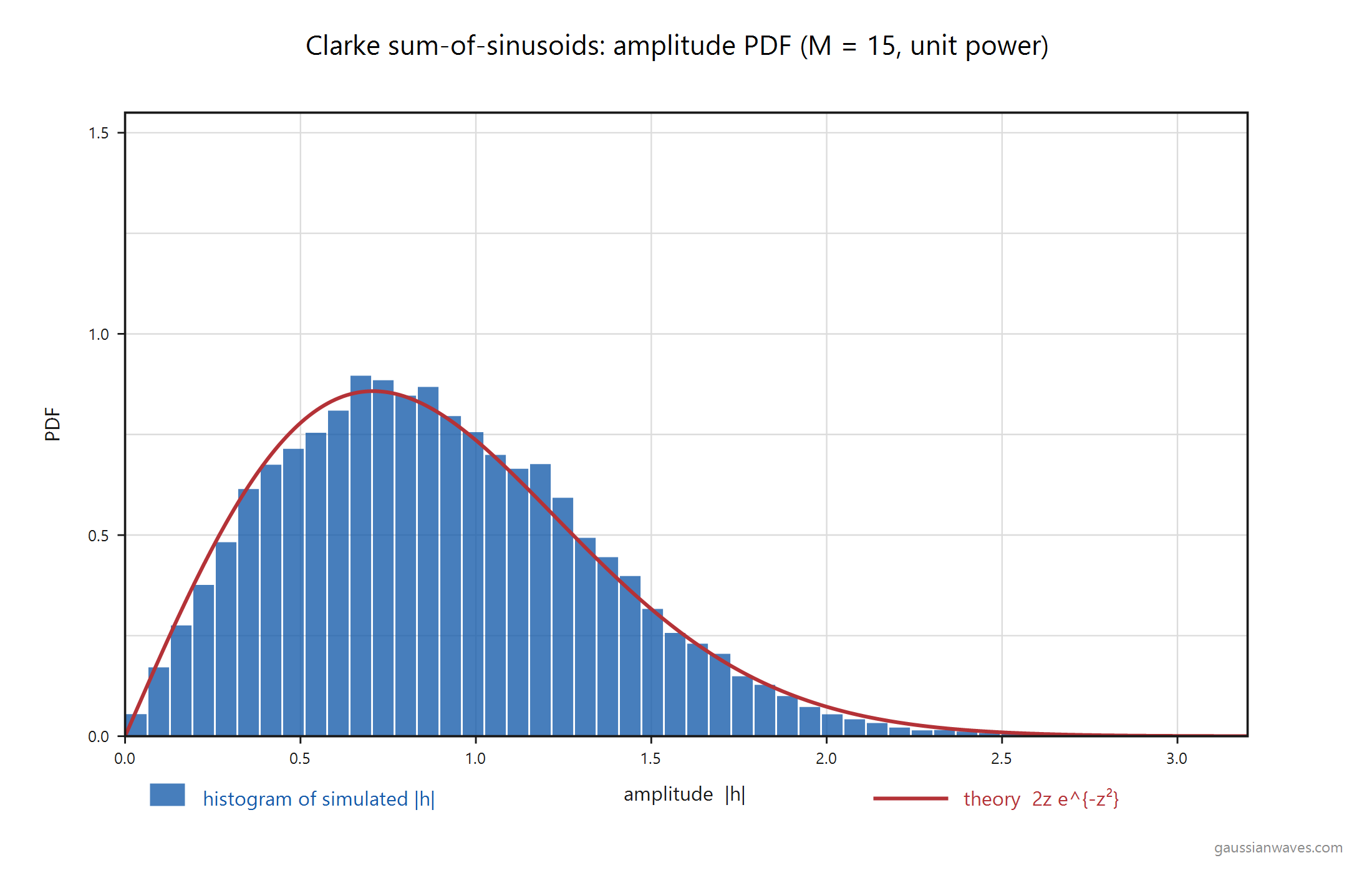
With \(M = 15\), \(N = 10^5\), \(f_D = 100\,\mathrm{Hz}\) and \(T_s = 10^{-4}\,\mathrm{s}\), the sample means of the quadratures sit near zero, each variance sits near \(1/2\), and the amplitude histogram follows the Rayleigh curve of unit power.
See also
[1] Eb/N0 Vs BER for BPSK over Rayleigh Channel and AWGN Channel
[2] Young’s model for Rayleigh fading
[3] MathWorks BER documentation
Python sketch: Rayleigh envelope from complex Gaussians
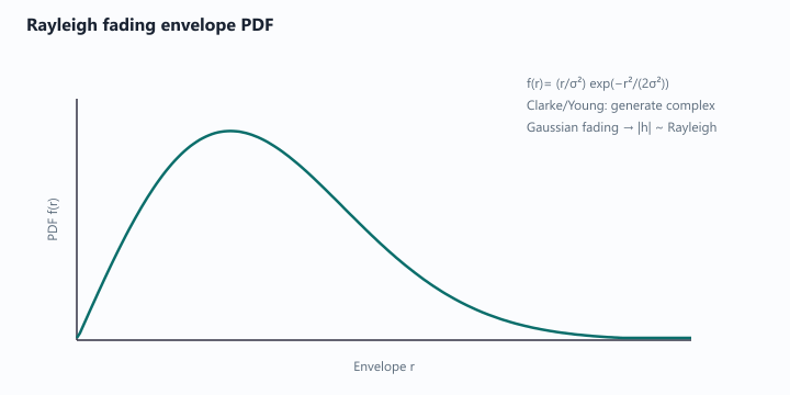
Clarke’s sum-of-sinusoids builds time-correlated \(h(t)\). The marginal distribution of a well-normalized isotropic complex Gaussian still has Rayleigh envelope:
import numpy as np

N = 200_000
h = (np.random.randn(N) + 1j*np.random.randn(N)) / np.sqrt(2)  # E[|h|^2]=1
r = np.abs(h)
# crude PDF check: mean of Rayleigh(σ=1/√2) is sqrt(π/4) ≈ 0.886
print('mean envelope ~', r.mean(), ' (theory 0.886)')
print('E[|h|^2] ~', np.mean(np.abs(h)**2))
For standardized 5G delay profiles after you leave flat fading, jump to the 3GPP TDL calculator and the TDL multipath article.
FAQ
What is the recommended reading order? Follow the six lessons at the top: Rayleigh BER → Clarke → Young → SIMO models → Selection combining → MRC. Optional branch: Rician fading.
How many multipaths is practical for simulating the channel?
thanks for help me
Hi,
When we generate time correlated channels using models like Jakes, Clarkes etc we also take the maximum doppler as a parameter.
When we consider finally modeling a channel as a FIR filter, before applying this filter to the data, depending on the doppler shift, is it required to multiply the time domain data with an exponential term or does the channel model take care of the frequency shift ?
basically we have x*exp(j2pi*delf*n/N) convolved with h = y
is jakes model finding a h’ such that x convolved with h’ mimics y ?
please help ….
Doppler spectrum is already available in the above implementation. No need to do additional multiplication of exponential factor. The equation above uses the max doppler spread as one of the parameters. When used, the model provides the expected Jake’s doppler spectrum.
I have bought your book and first of all I want to thank you for this useful working.I’m working on my thesis related to OFDM System on HF Channel. I learned useful informations from your book but I’d like to expect to see the sample Matlab code for OFDM system on Rayleigh channel. There is an example code in your book for AWGN channel, but I need Rayleigh channel with OFDM system. I want to use “rayleighchan” function in Matlab. Could you please help me regarding this topic? Do yu have any sample code for this issue?
I do not have the ready-made available for this scenario. But the ebook contains all the resources required for it.
The simplest thing is to model the Rayleigh multipath as statistical random variable. The chapter 6.3 in the ebook contains the simulation code for BPSK over Rayleigh Channel. Here, the Rayleigh channel is modeled statistically. The same can be integrated in the OFDM model given in Chapter 7.
Thanks a lot for your support.
Thank you for your support. I have a little question. Can I model the path delays, Doppler shifts of the each paths using statistical random variable model as specified in your book? I’d like to simulate 2,3 or 4 paths and change the path delays (1 ms, 5 ms, 10 ms etc.), Doppler shifts (1 Hz, 10 Hz, etc). Do I have to use the “rayleighchan” function for it? Thank you in advance.
Hi,
I have a question regarding above simulation code (also specified in your book), what is the delay spread in your above code? How can we add the delay spread into code?
Hi, great article!
Would you please be so kind to help me about my student project? I believe it’s a couple minutes for you.
Can you generate mathlab code for OFDM Double Rayleigh fading? It would help me a lot. Thank you.
Best regards.
please Sir Mathuranathan can you help me with small code matlab to generate the impulse response of rice channel?
sorry. I do not have code right now. I will add it in the queue for the future posts
Hi,
I work alone on my project of final year (enginner in telecommunications)
I have not found results about code of comparaison BICM and BICM-ID in the cannal AWGN and Rayleigh systems with matlab.
can you help me with small code matlab
Please.
I find this description slightly confusing.
The initial explanation is in terms of an L-tap FIR, L being the number of reflections, which makes inuitive sense. I was expecting a derivation for the FIR tap weights.
Instead, the derivation generates an overall impulse response which now requires a (complex) convolution to get the response to the input signal.
Is that right ?
y = x h
where is the convolution operator.
Which should end up being,
[real(x) real(h) – imag(x) imag(h)] + j[real(x) imag(h) + imag(x) real*h)]
which requires 4 N point convolutions.
Hello sir, when you have a power delay profile. We can simulate jakes model using PDP, by just multiplying the taps obtained from the PDP model to the coefficients obtained from jakes model .Is my approach correct?
It depends on the type of channel or in other words the surrounding environment you want to simulate. For, example for pedestrian users the extended pedestrian A model (EPA) is used in which the power delay profile (PDP) consists of 7 multipaths or if you want to simulate the vehicular environment then the EVA model s used in which the channel is simulated with 9 paths. While in ETU the number of paths are the same (9) as EVA channel.