Interpret FFT, complex DFT, frequency bins & FFTShift

Key focus: Interpret FFT results, complex DFT, frequency bins, fftshift and ifftshift. Know how to use them in analysis using Matlab and Python.

This article is part of the following books ● Digital Modulations using Matlab : Build Simulation Models from Scratch, ISBN: 978-1521493885 ● Digital Modulations using Python ISBN: 978-1712321638 ● Wireless communication systems in Matlab ISBN: 979-8648350779 All books available in ebook (PDF) and Paperback formats

Four types of Fourier Transforms:

Often, one is confronted with the problem of converting a time domain signal to frequency domain and vice-versa. Fourier Transform is an excellent tool to achieve this conversion and is ubiquitously used in many applications. In signal processing, a time domain signal can be continuous or discrete and it can be aperiodic or periodic. This gives rise to four types of Fourier transforms.

From Table 1, we note note that when the signal is discrete in one domain, it will be periodic in other domain. Similarly, if the signal is continuous in one domain, it will be aperiodic (non-periodic) in another domain. For simplicity, let’s not venture into the specific equations for each of the transforms above. We will limit our discussion to DFT, that is widely available as part of software packages like Matlab, Scipy(python) etc.., however we can approximate other transforms using DFT.

Real and Complex versions of transforms

For each of the listed transforms above, there exist a real version and complex version. The real version of the transform, takes in a real numbers and gives two sets of real frequency domain points – one set representing coefficients over \(cosine\) basis function and the other set representing the co-efficient over \(sine\) basis function. The complex version of the transforms represent positive and negative frequencies in a single array. The complex versions are flexible that it can process both complex valued signals and real valued signals. The following figure captures the difference between real DFT and complex DFT.

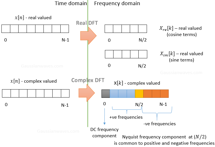
Real DFT:

Consider the case of N-point \(real\) DFT , it takes in N  samples of (real-valued) time domain waveform \(x[n]\) and gives two arrays of length \(N/2+1\) each set projected on cosine and sine functions respectively.

Here, the time domain index \(n\) runs from \(0 \rightarrow N\), the frequency domain index \(k\) runs from \(0 \rightarrow N/2\)

The real-valued time domain signal $\mathrm{x[n]}$ can be synthesized from the real DFT pairs as

Caveat: When using the synthesis equation, the values \(X_{re}[0]\) and \(X_{re}[N/2] \) must be divided by two. This problem is due to the fact that we restrict the analysis to real-values only. These type of problems can be avoided by using complex version of DFT.

Complex DFT:

Consider the case of N-point complex DFT, it takes in N samples of complex-valued time domain waveform \(x[n]\) and produces an array \(X[k]\) of length N.

The arrays values are interpreted as follows

● \(X[0]\) represents DC frequency component
● Next \(N/2\) terms are positive frequency components with \(X[N/2]\) being the Nyquist frequency (which is equal to half of sampling frequency)
● Next \(N/2-1\) terms are negative frequency components (note: negative frequency components are the phasors rotating in opposite direction, they can be optionally omitted depending on the application)

The corresponding synthesis equation (reconstruct \(x[n]\) from frequency domain samples \(X[k]\)) is

From these equations we can see that the real DFT is computed by projecting the signal on cosine and sine basis functions. However, the complex DFT projects the input signal on exponential basis functions (Euler’s formula connects these two concepts).

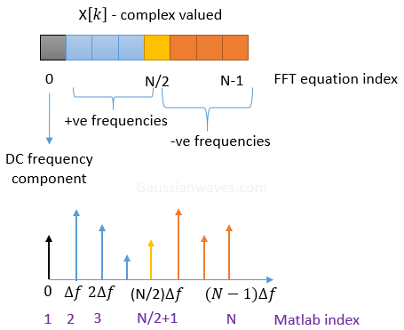
When the input signal in the time domain is real valued, the complex DFT zero-fills the imaginary part during computation (That’s its flexibility and avoids the caveat needed for real DFT). The following figure shows how to interpret the raw FFT results in Matlab that computes complex DFT. The specifics will be discussed next with an example.

Fast Fourier Transform (FFT)

The FFT function in Matlab  is an algorithm published in 1965 by J.W.Cooley and J.W.Tuckey for efficiently calculating the DFT. It exploits the special structure of DFT when the signal length is a power of 2, when this happens, the computation complexity is significantly reduced.  FFT length is generally considered as power of 2 – this is called \(radix-2\) FFT which exploits the twiddle factors. The FFT length can be odd as used in this particular FFT implementation – Prime-factor FFT algorithm where the FFT length factors into two co-primes.

FFT is widely available in software packages like Matlab, Scipy etc.., FFT in Matlab/Scipy implements the complex version of DFT. Matlab’s FFT implementation computes the complex DFT that is very similar to above equations except for the scaling factor. For comparison, the Matlab’s FFT implementation computes the complex DFT and its inverse as

The Matlab commands that implement the above equations are FFT and IFFT) respectively. The corresponding syntax is as follows

X = fft(x,N) %compute X[k]
x = ifft(X,N) %compute x[n]

Interpreting the FFT results

Lets assume that the \(x[n]\) is the time domain cosine signal of frequency \(f_c=10Hz\) that is sampled at a frequency \(f_s=32*fc\) for representing it in the computer memory.

fc=10;%frequency of the carrier
fs=32*fc;%sampling frequency with oversampling factor=32
t=0:1/fs:2-1/fs;%2 seconds duration
x=cos(2*pi*fc*t);%time domain signal (real number)
subplot(3,1,1); plot(t,x);hold on; %plot the signal
title('x[n]=cos(2 \pi 10 t)'); xlabel('n'); ylabel('x[n]');

Lets consider taking a \(N=256\) point FFT, which is the \(8^{th}\) power of \(2\).

N=256; %FFT size
X = fft(x,N);%N-point complex DFT
%output contains DC at index 1, Nyquist frequency at N/2+1 th index
%positive frequencies from index 2 to N/2
%negative frequencies from index N/2+1 to N

Note: The FFT length should be sufficient to cover the entire length of the input signal. If \(N\) is less than the length of the input signal, the input signal will be truncated when computing the FFT. In our case, the cosine wave is of 2 seconds duration and it will have 640 points (a \(10Hz\) frequency wave sampled at 32 times oversampling factor will have \(2 \times 32 \times 10 = 640\) samples in 2 seconds of the record). Since our input signal is periodic, we can safely use \(N=256\) point FFT, anyways the FFT will extend the signal when computing the FFT (see additional topic on spectral leakage that explains this extension concept).

Due to Matlab’s index starting at 1, the DC component of the FFT decomposition is present at index 1.

>>X(1)
 1.1762e-14   (approximately equal to zero)

That’s pretty easy. Note that the index for the raw FFT are integers from \(1 \rightarrow N\). We need to process it to convert these integers to \(frequencies\). That is where the \(sampling\) frequency counts.

Each point/bin in the FFT output array is spaced by the frequency resolution \(\Delta f\) that is calculated as

where, \(f_s\) is the sampling frequency and \(N\) is the FFT size that is considered. Thus, for our example, each point in the array is spaced by the frequency resolution

Now, the \(10 Hz\) cosine signal will leave a spike at the 8th sample (\(10/1.25=8\)), which is located at index 9 (See next figure).

>> abs(X(8:10)) %display samples 7 to 9
ans = 0.0000  128.0000    0.0000

Therefore, from the frequency resolution, the entire frequency axis can be computed as

%calculate frequency bins with FFT
df=fs/N %frequency resolution
sampleIndex = 0:N-1; %raw index for FFT plot
f=sampleIndex*df; %x-axis index converted to frequencies

Now we can plot the absolute value of the FFT against frequencies as

subplot(3,1,2); stem(sampleIndex,abs(X)); %sample values on x-axis
title('X[k]'); xlabel('k'); ylabel('|X(k)|');
subplot(3,1,3); plot(f,abs(X)); %x-axis represent frequencies
title('X[k]'); xlabel('frequencies (f)'); ylabel('|X(k)|');

The following plot shows the frequency axis and the sample index as it is for the complex FFT output.

After the frequency axis is properly transformed with respect to the sampling frequency, we note that the cosine signal has registered a spike at \(10 Hz\). In addition to that, it has also registered a spike at \(256-8=248^{th}\) sample that belongs to negative frequency portion. Since we know the nature of the signal, we can optionally ignore the negative frequencies. The sample at the Nyquist frequency (\(f_s/2\)) mark the boundary between the positive and negative frequencies.

>> nyquistIndex=N/2+1;
>> X(nyquistIndex-2:nyquistIndex+2).'
ans =
1.0e-13 *
  -0.2428 + 0.0404i
  -0.1897 + 0.0999i
  -0.3784          
  -0.1897 - 0.0999i
  -0.2428 - 0.0404i

Note that the complex numbers surrounding the Nyquist index are complex conjugates and they represent positive and negative frequencies respectively.

FFTShift

From the plot we see that the frequency axis starts with DC, followed by positive frequency terms which is in turn followed by the negative frequency terms. To introduce proper order in the x-axis, one can use FFTshift function Matlab, which arranges the frequencies in order: negative frequencies \(\rightarrow\) DC \(\rightarrow\) positive frequencies. The fftshift function need to be carefully used when \(N\) is odd.

For even N, the original order returned by FFT  is as follows (note: all indices below corresponds to Matlab’s index)

● \(X[1]\) represents DC frequency component
● \(X[2]\) to \(X[N/2]\) terms are positive frequency components
● \(X[N/2+1]\) is the Nyquist frequency (\(F_s/2\)) that is common to both positive and negative frequencies. We will consider it as part of negative frequencies to have the same equivalence with the fftshift function.
● \(X[N/2+1]\) to \(X[N]\) terms are considered as negative frequency components

FFTshift shifts the DC component to the center of the spectrum. It is important to remember that the Nyquist frequency at the (N/2+1)th Matlab index is common to both positive and negative frequency sides. FFTshift command puts the Nyquist frequency in the negative frequency side. This is captured in the following illustration.

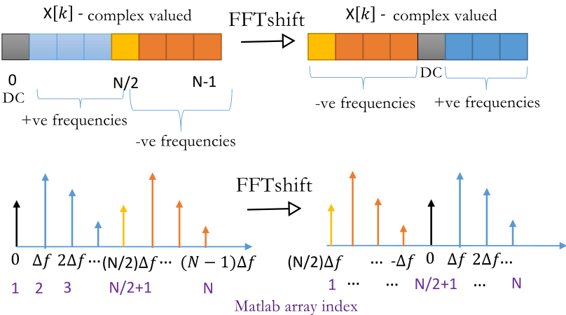
Therefore, when \(N\) is even, ordered frequency axis is set as

When (N) is odd, the ordered frequency axis should be set as

The following code snippet, computes the fftshift using both the manual method and using the Matlab’s in-build command. The results are plotted by superimposing them on each other. The plot shows that both the manual method and fftshift method are in good agreement.

%two-sided FFT with negative frequencies on left and positive frequencies on right
%following works only if N is even, for odd N see equation above
X1 = [(X(N/2+1:N)) X(1:N/2)]; %order frequencies without using fftShift
X2 = fftshift(X);%order frequencies by using fftshift

df=fs/N; %frequency resolution
sampleIndex = -N/2:N/2-1; %raw index for FFT plot
f=sampleIndex*df; %x-axis index converted to frequencies
%plot ordered spectrum using the two methods
figure;subplot(2,1,1);stem(sampleIndex,abs(X1));hold on; stem(sampleIndex,abs(X2),'r') %sample index on x-axis
title('Frequency Domain'); xlabel('k'); ylabel('|X(k)|');%x-axis represent sample index
subplot(2,1,2);stem(f,abs(X1)); stem(f,abs(X2),'r') %x-axis represent frequencies
xlabel('frequencies (f)'); ylabel('|X(k)|');

Comparing the bottom figures in the Figure 4 and Figure 6, we see that the ordered frequency axis is more meaningful to interpret.

IFFTShift

One can undo the effect of fftshift by employing ifftshift function. The ifftshift function restores the raw frequency order. If the FFT output is ordered using fftshift function, then one must restore the frequency components back to original order BEFORE taking IFFT. Following statements are equivalent.

X = fft(x,N) %compute X[k]
x = ifft(X,N) %compute x[n]

X = fftshift(fft(x,N)); %take FFT and rearrange frequency order (this is mainly done for interpretation)
x = ifft(ifftshift(X),N)% restore raw frequency order and then take IFFT

Some observations on FFTShift and IFFTShift

When \(N\) is odd and for an arbitrary sequence, the fftshift and ifftshift functions will produce different results. However, when they are used in tandem, it restores the original sequence.

>>  x=[0,1,2,3,4,5,6,7,8]
0     1     2     3     4     5     6     7     8
>>  fftshift(x)
5     6     7     8     0     1     2     3     4
>>  ifftshift(x)
4     5     6     7     8     0     1     2     3
>>  ifftshift(fftshift(x))
0     1     2     3     4     5     6     7     8
>>  fftshift(ifftshift(x))
0     1     2     3     4     5     6     7     8

When \(N\) is even and for an arbitrary sequence, the fftshift and ifftshift functions will produce the same result. When they are used in tandem, it restores the original sequence.

>>  x=[0,1,2,3,4,5,6,7]
0     1     2     3     4     5     6     7
>>  fftshift(x)
4     5     6     7     0     1     2     3
>>  ifftshift(x)
4     5     6     7     0     1     2     3
>>  ifftshift(fftshift(x))
0     1     2     3     4     5     6     7
>>  fftshift(ifftshift(x))
0     1     2     3     4     5     6     7

For Python code, please check the following book: Digital Modulations using Python – by Mathuranathan Viswanathan

Rate this article: (106 votes, average: 4.52 out of 5)

Topics in this chapter

Essentials of Signal Processing ● Generating standard test signals  □ Sinusoidal signals  □ Square wave  □ Rectangular pulse  □ Gaussian pulse  □ Chirp signal ● Interpreting FFT results - complex DFT, frequency bins and FFTShift  □ Real and complex DFT  □ Fast Fourier Transform (FFT)  □ Interpreting the FFT results  □ FFTShift  □ IFFTShift ● Obtaining magnitude and phase information from FFT  □ Discrete-time domain representation  □ Representing the signal in frequency domain using FFT  □ Reconstructing the time domain signal from the frequency domain samples ● Power spectral density ● Power and energy of a signal  □ Energy of a signal  □ Power of a signal  □ Classification of signals  □ Computation of power of a signal - simulation and verification ● Polynomials, convolution and Toeplitz matrices  □ Polynomial functions  □ Representing single variable polynomial functions  □ Multiplication of polynomials and linear convolution  □ Toeplitz matrix and convolution ● Methods to compute convolution  □ Method 1: Brute-force method  □ Method 2: Using Toeplitz matrix  □ Method 3: Using FFT to compute convolution  □ Miscellaneous methods ● Analytic signal and its applications  □ Analytic signal and Fourier transform  □ Extracting instantaneous amplitude, phase, frequency  □ Phase demodulation using Hilbert transform ● Choosing a filter : FIR or IIR : understanding the design perspective  □ Design specification  □ General considerations in design

Books by the author

Wireless Communication Systems in Matlab Second Edition(PDF) Note: There is a rating embedded within this post, please visit this post to rate it. $14.99 – Add to Cart Checkout Added to cart	Digital Modulations using Python (PDF ebook) Note: There is a rating embedded within this post, please visit this post to rate it. $14.99 – Add to Cart Checkout Added to cart	Digital Modulations using Matlab (PDF ebook) Note: There is a rating embedded within this post, please visit this post to rate it. $14.99 – Add to Cart Checkout Added to cart
Hand-picked Best books on Communication Engineering Best books on Signal Processing