RMS Formula: Root Mean Square of a Signal Explained

Energy & Spectra (same on every page in this path)

1. Power & energy → 2. Parseval → 3. RMS value (you are here)

In one sentence: The RMS formula is the square root of the mean of $|x|^2$ — the equivalent DC value that delivers the same average power into a resistor as the original waveform.

Matlab/Python simulation: Apply the discrete RMS formula to sampled vectors in Matlab or NumPy when you estimate signal power; pair it with power & energy of a signal and Parseval’s theorem.

Root Mean Square (RMS) value is one of the most important parameters that signifies the size of a signal.

Defining the term “size”:

In signal processing, a signal is viewed as a function of time. The term “size of a signal” is used to represent “strength of the signal”. It is crucial to know the “size” of a signal used in a certain application. For example, we may be interested to know the amount of electricity needed to power an LCD monitor as opposed to a CRT monitor. Both of these applications are different and have different tolerances. Thus the amount of electricity driving these devices will also be different.

A given signal’s size can be measured in many ways. Some of them are:

Total energy
Square root of total energy
Integral absolute value
Maximum or peak absolute value
Root Mean Square (RMS) value
Average Absolute (AA) value

Parseval’s theorem: rms formula

Parseval’s theorem expresses the energy of a signal in the time domain in terms of the average energy in its frequency components.

Suppose $x[n]$ is a sequence of complex numbers of length $N$, $x[n] = {x_0, x_1, \ldots, x_{N-1}}$. Its $N$-point discrete Fourier transform (DFT) $X[k]$ is

$$X[k] = \sum_{n=0}^{N-1} x[n]\, e^{-j\frac{2\pi}{N} k n}$$

The inverse discrete Fourier transform is

$$x[n] = \frac{1}{N} \sum_{k=0}^{N-1} X[k]\, e^{j\frac{2\pi}{N} k n}$$

Suppose $x[n]$ and $y[n]$ are two such sequences that follow the above definitions. Parseval’s theorem is written as

$$\boxed{ \displaystyle{\sum_{n=0}^{N-1} x[n]\, y^{\ast}[n] = \frac{1}{N} \sum_{k=0}^{N-1} X[k]\, Y^{\ast}[k]}}$$

where $\ast$ indicates the complex conjugate.

Deriving Parseval’s theorem

$$\begin{aligned} \sum_{n=0}^{N-1} x[n]\, y^{\ast}[n] &= \sum_{n=0}^{N-1} x[n] \left(\frac{1}{N} \sum_{k=0}^{N-1} Y[k]\, e^{j\frac{2\pi}{N} k n} \right)^{\ast} \\ &= \frac{1}{N} \sum_{n=0}^{N-1} x[n] \sum_{k=0}^{N-1} Y^{\ast}[k]\, e^{-j\frac{2\pi}{N} k n} \\ &= \frac{1}{N} \sum_{k=0}^{N-1} Y^{\ast}[k] \cdot \sum_{n=0}^{N-1} x[n]\, e^{-j\frac{2\pi}{N} k n} \\ &= \frac{1}{N} \sum_{k=0}^{N-1} X[k]\, Y^{\ast}[k] \end{aligned}$$

Energy content

Given a discrete-time sequence of length $N$, $x[n] = {x_0, x_1, \ldots, x_{N-1}}$, Parseval’s theorem says that the energy content of the signal in the time domain equals the average of the energy contained in its frequency components.

For any complex sample, $x[n]\, x^{\ast}[n] = |x[n]|^2$, so setting $y = x$ in the theorem gives

$$\boxed{ \displaystyle{\sum_{n=0}^{N-1} \left| x[n] \right|^2 = \frac{1}{N} \sum_{k=0}^{N-1} \left| X[k] \right|^2 }}$$

Mean Square value

The mean square value is the arithmetic mean of the squares of a given set of numbers. For a complex-valued signal represented by $N$ discrete samples ${x_0, x_1, \ldots, x_{N-1}}$, the mean square value $x_{MS}$ is

$$x_{MS} = \frac{|x_0|^2 + |x_1|^2 + \cdots + |x_{N-1}|^2}{N} = \frac{1}{N} \sum_{n=0}^{N-1} |x[n]|^2$$

Applying Parseval’s theorem, the mean square value can also be computed from the frequency-domain components $X[k]$:

$$x_{MS} : \quad \frac{1}{N} \sum_{n=0}^{N-1} |x[n]|^2 = \frac{1}{N^2} \sum_{k=0}^{N-1} \left| X[k] \right|^2$$

RMS value

The RMS value of a signal is the square root of the average of its squared values. For a complex-valued signal represented by $N$ discrete samples, the RMS value $x_{RMS}$ is

$$x_{RMS} = \sqrt{\frac{|x_0|^2 + |x_1|^2 + \cdots + |x_{N-1}|^2}{N}} = \sqrt{\frac{1}{N} \sum_{n=0}^{N-1} |x[n]|^2}$$

Applying Parseval’s theorem, the RMS value can also be computed from the frequency-domain components $X[k]$:

$$x_{RMS} : \quad \sqrt{\frac{1}{N} \sum_{n=0}^{N-1} |x[n]|^2} = \sqrt{\frac{1}{N^2} \sum_{k=0}^{N-1} \left| X[k] \right|^2}$$

Implementing in Matlab

The following Matlab code computes the RMS value of a random sequence in the time domain and in the frequency domain, using Parseval’s theorem. Figure 1 shows the RMS values of some well-known waveforms.

rng(1);                                   % fixed seed so the result is reproducible
N = 100;                                  % length of the signal
x = randn(1,N);                           % a random signal to test
X = fft(x);                               % frequency-domain representation

RMS1 = sqrt(mean(x.*conj(x)))             % RMS from time-domain samples
RMS2 = sqrt(sum(X.*conj(X))/length(x)^2)  % RMS from the DFT (Parseval)
RMS3 = rms(x)                             % built-in function

% Result: RMS1 = RMS2 = RMS3 = 0.9913

rng(1);                                   % fixed seed so the result is reproducible
N = 100;                                  % length of the signal
x = randn(1,N);                           % a random signal to test
X = fft(x);                               % frequency-domain representation

RMS1 = sqrt(mean(x.*conj(x)))             % RMS from time-domain samples
RMS2 = sqrt(sum(X.*conj(X))/length(x)^2)  % RMS from the DFT (Parseval)
RMS3 = rms(x)                             % built-in function

% Result: RMS1 = RMS2 = RMS3 = 0.9913

Both time-domain and frequency-domain approaches give the same value, and the built-in rms function agrees.

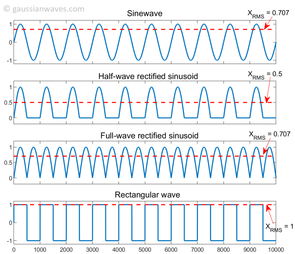
Figure 1: RMS values of some well-known signals: sinewave (0.707), half-wave rectified sinusoid (0.5), full-wave rectified sinusoid (0.707) and rectangular wave (1).

Implementing in Python

The same two calculations with NumPy’s FFT routines:

import numpy as np

rng = np.random.default_rng(1)
N = 100
x = rng.standard_normal(N)                       # random test signal
X = np.fft.fft(x)                                # N-point DFT

rms_time = np.sqrt(np.mean(np.abs(x)**2))        # from time samples
rms_freq = np.sqrt(np.sum(np.abs(X)**2) / N**2)  # from the DFT (Parseval)

print(f"RMS (time) = {rms_time:.4f}")
print(f"RMS (freq) = {rms_freq:.4f}")

import numpy as np

rng = np.random.default_rng(1)
N = 100
x = rng.standard_normal(N)                       # random test signal
X = np.fft.fft(x)                                # N-point DFT

rms_time = np.sqrt(np.mean(np.abs(x)**2))        # from time samples
rms_freq = np.sqrt(np.sum(np.abs(X)**2) / N**2)  # from the DFT (Parseval)

print(f"RMS (time) = {rms_time:.4f}")
print(f"RMS (freq) = {rms_freq:.4f}")

Expected output: RMS (time) = 0.8547 and RMS (freq) = 0.8547.

Significance of RMS value

► One of the most important parameters used to describe the strength of an Alternating Current (AC).

► The RMS value of an AC voltage or current is equivalent to the DC voltage or current that produces the same heating effect when applied across an identical resistor. Hence, it is also a measure of the energy content of a given signal.

► In statistics, for any zero-mean random stationary signal, the RMS value is the same as the standard deviation of the signal. Example: the RMS delay spread of a multipath channel is the standard deviation of the excess delays, weighted by the power delay profile (PDP). With PDP powers $P_k$ at delays $\tau_k$:

$$\tau_{\mathrm{rms}}=\sqrt{\frac{\sum_k P_k\tau_k^2}{\sum_k P_k}-\left(\frac{\sum_k P_k\tau_k}{\sum_k P_k}\right)^2}$$

► When two uncorrelated (zero cross-correlation) signals are added together, such as noise from two independent sources, the RMS value of their sum is the square root of the sum of the squares of their individual RMS values.

FAQ

What is the RMS value of a sine wave with amplitude A? For $x(t)=A\sin(\omega t)$, the RMS value is $A/\sqrt{2}\approx 0.707A$. That is why AC voltmeters often report RMS, and why “120 V RMS” is not a peak voltage.

How does RMS relate to average power? Into a 1 Ω resistor, average power equals $(\mathrm{RMS})^2$. More generally, RMS is the DC-equivalent magnitude that delivers the same average power as the original waveform into a resistive load.

How do I compute RMS for a discrete block of samples? Use $\sqrt{\frac{1}{N}\sum_{n=0}^{N-1}|x[n]|^2}$. That is exactly the square root of the block’s average power (with the usual 1 Ω normalized-signal convention in DSP).

Root Mean Square (RMS) Formula Explained for Signals