Key focus: Learn how to use Hilbert transform to extract envelope, instantaneous phase and frequency from a modulated signal. Hands-on demo using Python & Matlab.
If you would like to brush-up the basics on analytic signal and how it related to Hilbert transform, you may visit article: Understanding Analytic Signal and Hilbert Transform
Introduction
The concept of instantaneous amplitude/phase/frequency are fundamental to information communication and appears in many signal processing application. We know that a monochromatic signal of form $latex x(t) = a cos(\omega t + \phi)$ cannot carry any information. To carry information, the signal need to be modulated. Take for example the case of amplitude modulation, in which a positive real-valued signal $latex m(t)$ modulates a carrier $latex cos(\omega_c t)$. That is, the amplitude modulation is effected by multiplying the information bearing signal $latex m(t)$ with the carrier signal $latex cos(\omega_c t)$.
$latex x(t) = m(t) cos\left(\omega_c t\right) &s=2$
Here, $latex \omega_c$ is the angular frequency of the signal measured in radians/sec and is related to the temporal frequency $latex f_c$ as $latex \omega_c = 2 \pi f_c$. The term $latex m(t)$ is also called instantaneous amplitude.
Similarly, in the case of phase or frequency modulations, the concept of instantaneous phase or instantaneous frequency is required for describing the modulated signal.
$latex x(t) = a cos \left(\phi(t) \right) &s=2$
Here, $latex a$ is the constant amplitude factor (no change in the envelope of the signal) and $latex \phi(t)$ is the instantaneous phase which varies according to the information. The instantaneous angular frequency is expressed as the derivative of instantaneous phase.
$latex \begin{aligned} \omega(t) &= \frac{d}{dt} \phi(t) \ f(t) &= \frac{1}{2 \pi} \frac{d}{dt} \phi(t) \end{aligned}&s=2$
[table “47” not found /]
Definition
Generalizing these concepts, if a signal is expressed as $latex x(t) = a(t) cos \left[ \phi (t) \right] $
- The instantaneous amplitude or the envelope of the signal is given by $latex a(t)$
- The instantaneous phase is given by $latex \phi(t)$
- The instantaneous angular frequency is derived as $latex \omega(t) = \frac{d}{dt} \phi(t)$
- The instantaneous temporal frequency is derived as $latex f(t) = \frac{1}{2 \pi} \frac{d}{dt} \phi(t) $
Problem statement
An amplitude modulated signal is formed by multiplying a sinusoidal information and a linear frequency chirp. The information content is expressed as $latex a(t) = 1 + 0.7 \; sin \left( 2 \pi 3 t\right)$ and the linear frequency chirp is made to vary from $latex 20 \; Hz$ to $latex 80 \; Hz$. Given the modulated signal, extract the instantaneous amplitude (envelope), instantaneous phase and the instantaneous frequency.
Solution
We note that the modulated signal is a real-valued signal. We also take note of the fact that amplitude/phase and frequency can be easily computed if the signal is expressed in complex form. Which transform should we use such that the we can convert a real signal to the complex plane without altering the required properties ?? Answer: Apply Hilbert transform and form the analytic signal on the complex plane. Figure 1 illustrates this concept.

If we express the real-valued modulated signal $latex x(t)$ as an analytic signal, it is expressed in complex plane as
$latex z(t) = z_r(t) + j z_i(t) = x(t) + j HT \left[ x(t) \right] &s=2$
where, (HT[.]) represents the Hilbert Transform operation. Now, the required parameters are very easy to obtain.
The instantaneous amplitude (envelope extraction) is computed in the complex plane as
$latex a(t) = |z(t)| = \sqrt{z_r^2(t) + z_i^2(t)} &s=2$
The instantaneous phase is computed in the complex plane as
$latex \phi(t) = \angle z(t) = arctan \left[ \frac{z_i(t)}{z_r(t)} \right] &s=2$
The instantaneous temporal frequency is computed in the complex plane as
$latex f(t) = \frac{1}{2 \pi} \frac{d}{dt} \phi(t) &s=2$
Once we know the instantaneous phase, the carrier can be regenerated as $latex cos[\phi(t)]$. The regenerated carrier is often referred as Temporal Fine Structure (TFS) in Acoustic signal processing [1].
Matlab
fs = 600; %sampling frequency in Hz
t = 0:1/fs:1-1/fs; %time base
a_t = 1.0 + 0.7 * sin(2.0*pi*3.0*t) ; %information signal
c_t = chirp(t,20,t(end),80); %chirp carrier
x = a_t .* c_t; %modulated signal
subplot(2,1,1); plot(x);hold on; %plot the modulated signal
z = hilbert(x); %form the analytical signal
inst_amplitude = abs(z); %envelope extraction
inst_phase = unwrap(angle(z));%inst phase
inst_freq = diff(inst_phase)/(2*pi)*fs;%inst frequency
%Regenerate the carrier from the instantaneous phase
regenerated_carrier = cos(inst_phase);
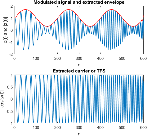
plot(inst_amplitude,'r'); %overlay the extracted envelope
title('Modulated signal and extracted envelope'); xlabel('n'); ylabel('x(t) and |z(t)|');
subplot(2,1,2); plot(cos(inst_phase));
title('Extracted carrier or TFS'); xlabel('n'); ylabel('cos[\omega(t)]');Python
import numpy as np
from scipy.signal import hilbert, chirp
import matplotlib.pyplot as plt

fs = 600.0 #sampling frequency
duration = 1.0 #duration of the signal
t = np.arange(int(fs*duration)) / fs #time base

a_t =  1.0 + 0.7 * np.sin(2.0*np.pi*3.0*t)#information signal
c_t = chirp(t, 20.0, t[-1], 80) #chirp carrier
x = a_t * c_t #modulated signal

plt.subplot(2,1,1)
plt.plot(x) #plot the modulated signal

z= hilbert(x) #form the analytical signal
inst_amplitude = np.abs(z) #envelope extraction
inst_phase = np.unwrap(np.angle(z))#inst phase
inst_freq = np.diff(inst_phase)/(2*np.pi)*fs #inst frequency

#Regenerate the carrier from the instantaneous phase
regenerated_carrier = np.cos(inst_phase)

plt.plot(inst_amplitude,'r'); #overlay the extracted envelope
plt.title('Modulated signal and extracted envelope')
plt.xlabel('n')
plt.ylabel('x(t) and |z(t)|')
plt.subplot(2,1,2)
plt.plot(regenerated_carrier)
plt.title('Extracted carrier or TFS')
plt.xlabel('n')
plt.ylabel('cos[\omega(t)]')
Results
Rate this article: [ratings]
Reference
Topics in this chapter
[table “31” not found /]Books by the author
[table “23” not found /]
Great article! It helped me to understand better how Hilbert Transform works, but I have a doubt about the instantaneous phase. Applying a modulating signal m(t) in a carrier cossine (doing the Phase Modulation) like this: x(t) = Cos(wt + m(t)), where w = 2*pi*f and t = time. If I use the Hilbert Transform to get the instantaneous phase of the analytic signal using the commands in matlab:
z = hilbert(x);
inst_phase = unwrap(angle(z));
phase = inst_phase – wt;
Am I demodulating the signal x(t) and getting just the signal m(t)? If I am not doing it, what should I do to demodulate a signal in phase after apply the Hilbert Transform? Thank you very much for the help!! 🙂
You are absolutely right. What you have described is the essence of phase demodulation using hilbert transform. May be I can draft another article with Matlab examples for others to understand. Thanks for your comment.
Hey Mathuranathan! First or all, thank you very much for your reply! Oh yes! It would be really great if you could make another article with Matlab examples of Phase Demodulation using the Hilbert Transform. I am using that code on Matlab and using some modulating signals m(t) like cossines, square waves and Sawtooth waves just for examples of Phase Modulation/Demodulation, but, unfortunetely, I just can extract a line when I plot the phase signal.
Once again, thank you very much to share this knowledge for us:)
Here you go
https://www.gaussianwaves.com/2017/06/phase-demodulation-using-hilbert-transform-application-of-analytic-signal/
Hi, Thanks to your explanation. I have a question that if I have a signal which is composed of many harmonic frequencies, is it possible to use Hilbert transform to see some information from it?
Hilbert transform has wide range of applications. Two of them are listed here
Electrocardiography: The Hilbert transform is a widely used tool in interpreting electrocardiograms (ECGs).
The Hilbert-Huang transform: In time series analysis the Fourier transform is the dominating tool. However, this method is not good enough for nonstationary or nonlinear data. For this purpose, the Hilbert-Huang transform (HHT) was proposed. This method has gained popularity and is widely used in spectral analysis since it, in contrast to common ”Fourier methods”, suppose that frequency and amplitude of the harmonics are dependent on time. This is achieved by decomposing the time series into so called intrinsic mode functions (IMFs). However, in spite of considerable efforts, the HHT to this day lacks mathematical framework and the method is entirely empirical. Thus, the investigation of this method is carried out numerically in this thesis to try to understand how the method works and what limitations are inherit.
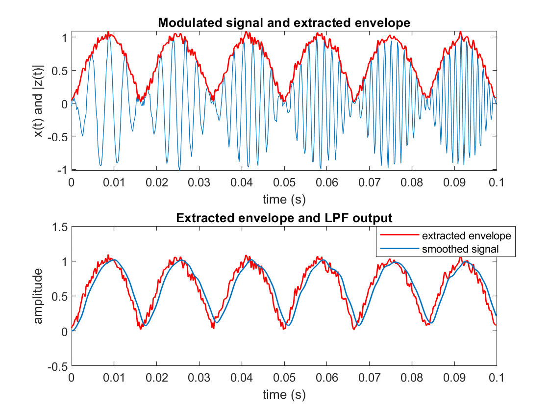
Can the envelope be smoothed? , if the answer I would like you to help me please
The extracted envelope can be smoothed by passing it through a low pass filter (LPF).
Use Matlab’s firpm function or Python Scipy’s remez function to design the LPF.
In the following example, I have added noise to the modulated signal and hence the extracted envelope is noisy. The noisy extracted envelope is passed through a LPF to obtain the smoothed signal.
Hi, Thank you very much for the great explanation, but I can not see the whole formula , could you please send me a .pdf or word copy? Thank you very much.
Thank you for letting me know. The formula display issue is corrected now.
I now understand clearly how to get ‘instantaneous phases’ of my data using matlab hilbert.m (z = hilbert(x)).
On my data, sliding window measurement (1 min time bin) of ‘instantaneous phases’ of brain voxel waves will yield, for example 84, phases for a bin,and the next bin will yield another 84 phases, and so on, to the last 280th time bin. Now, I need to confirm that the last phase (radian) of the previous time bin be equal to the first phase of the next time bin. As ‘unwrap’ was used to get ‘inst_phase = unwrap(angle(z)’ stiching phases of each seqential bin is OK without any touch such as shift?
p.s. While mouse roaming, inadvertantly rating was done and system does not allow me to change my rating even I once out and in again with this message “You Had Already Rated This Post. Post ID #14208.” Sorry for under-rating as rating should have been 5.00 from my side.
No problem. Thanks for the comment.
I had two questions if anyone can help me with it, if I want to find the envelope of signal which is not modulated what changes do I need to make in the python code provided. I tried to remove the chirp() statement and I didn’t multiply c_t, so x=a_t only. But I am not getting the correct answer.
Another question is say I want to provide a .wav file and not take input like the one shown, what changes do I need to make?
Hello! This article helped me a lot on signal processing, I am trying to develop an open source DSC decoder (FSK 100 baud, like Sitor-B), as there are only freeware, but closed source apps and only for Windows.
In general all is well, but I ran into problem when signal is framed, i.e. arrives in pieces, shorter than the actual DSC message (~9 s). Surely, PCs are powerful and have a lot of RAM these days and by detecting the start I could simply cache enough samples for full one message processing, but, well, I would like to make it work even with joined signals.
So the problem is, that if I process signal e.g. in 1 s frames, my instanteneous frequency does not join nicely. I tried to add a 0.1 s or 0.2 s overlap, but to no avail, I get false center frequency crossings.
Would you have any suggestion, how to join instant frequency response?
I currently do first Hilbert transform, then instantaneous phase and instanteneous frequency for all received frame. I also apply Butterworth filter on final “reconstructed” signal, but it jumps up and down where two frames meet. I.e. the start of the signal is sketchy. And even overlap with previous frame does not alleviate the issue. Maybe there is a better method of tracking instant frequency on such a running signal, doing it maybe just one-by-one sample?