Two ray ground reflection model

Friis propagation model considers the line-of-sight (LOS) path between the transmitter and the receiver. The expression for the received power becomes complicated if the effect of reflections from the earth surface has to be incorporated in the modeling. In addition to the line-of-sight path, a single reflected path is added in the two ray ground reflection model, as illustrated in Figure 1. This model takes into account the phenomenon of reflection from the ground and the antenna heights above the ground. The ground surface is characterized by reflection coefficient – $latex R$ which depends on the material properties of the surface and the type of wave polarization. The transmitter and receiver antennas are of heights $latex h_t$ and $latex h_r$ respectively and are separated by the distance of $latex d$ meters.

[table id=36/]

The received signal consists of two components: LOS ray that travels the free space from the transmitter and a reflected ray from the ground surface. The distances traveled by the LOS ray and the reflected ray are given by

Depending on the phase difference ($latex \phi$) between the LOS ray and reflected ray, the received signal may suffer constructive or destructive interference. Hence, this model is also called as two ray interference model.

where, $latex \lambda$ is the wavelength of the radiating wave that can be calculated from the transmission frequency. Under large-scale assumption, the power of the received signal can be expressed as

where $latex \sqrt{G_{los}}=\sqrt{G_a G_b}$ is the product of antenna field patterns along the LOS direction and $latex \sqrt{G_{los}}=\sqrt{G_c G_d}$ is the product of antenna field patterns along the reflected path.

The following piece of code implements equation 3 and plots the received power ($latex P_r$) against the separation distance ($latex d$). The resulting plot for $latex f=900\;MHz$, $latex R=-1$, $latex h_t=50\;m$, $latex h_r=2\;m$, $latex G_{los}=G_{ref}=1$ is shown in the Figure 2. In this plot, the transmitter power is normalized such that the plot starts at $latex 0\;dBm$. The plot also contains approximations of the received power over three regions.

twoRayModel.m: Two ray ground reflection model simulation (refer book for Matlab code – click here)

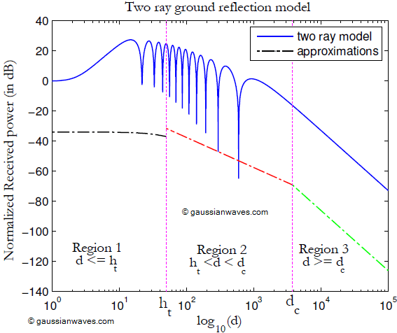
** the approximations are shifted down in the plot for clarity, otherwise they will ride on top of the two ray model

The distance that is denoted as $latex d_c$ in the plot, is called the critical distance. It is calculated $latex d_c=4 h_t h_r/\lambda$. For the region beyond the critical distance, the received power falls-off at $latex -40\;dB/decade$ rate. For the region where $latex h_t \leq d \leq d_c$, the received power falls-off at $latex -20\;dB/decade$ rate and it can be approximated by free space loss equation. Table 1 captures the approximate expressions that can be applied for the three distinct regions of propagation as identified in the plot above.

Rate this article: [ratings]

Topic in this chapter

• Introduction to Large scale propagation models
• Friis free space propagation model
• Log distance path loss model
• Two ray ground reflection model
• Modeling diffraction loss
  • Single knife-edge diffraction model
  • Fresnel zones
• Hata Okumura model for outdoor propagation

Books by the author

[table id=23 /]