
Articles in this series
- Phased array antenna — an introduction
- Electronic scanning arrays
- Grating lobes in electronic scanning
- Array pattern multiplication (this article)
Introduction
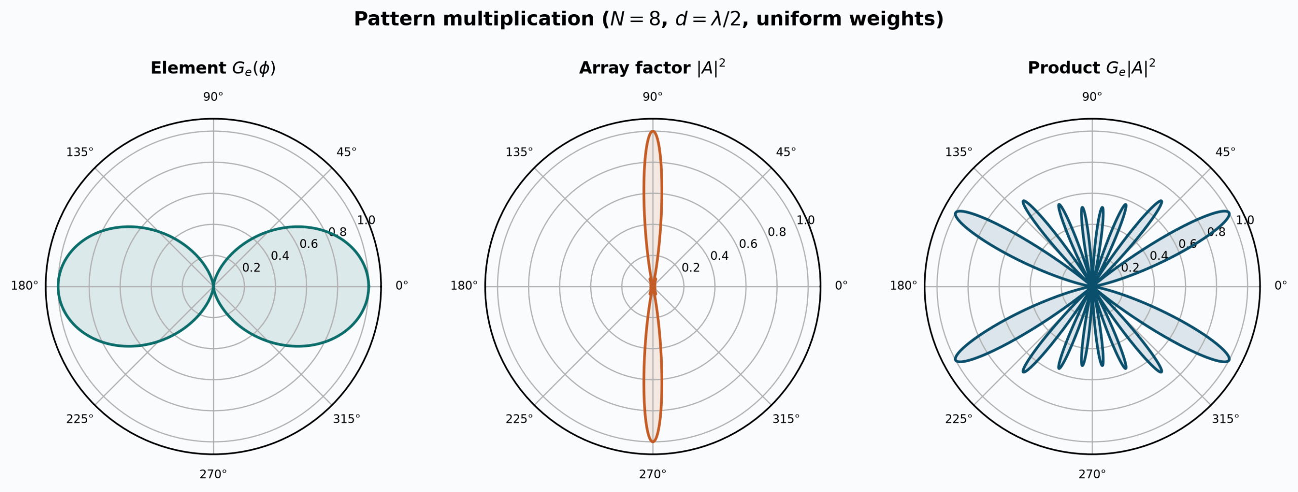
So far the radiators were mathematical points. Real dipoles and patches have their own angular patterns. If the elements are identical and oriented the same way, the total far-field pattern factors as element factor times array factor. Amplitude tapering then windows the discrete aperture to bring the sidelobes down.
Motive
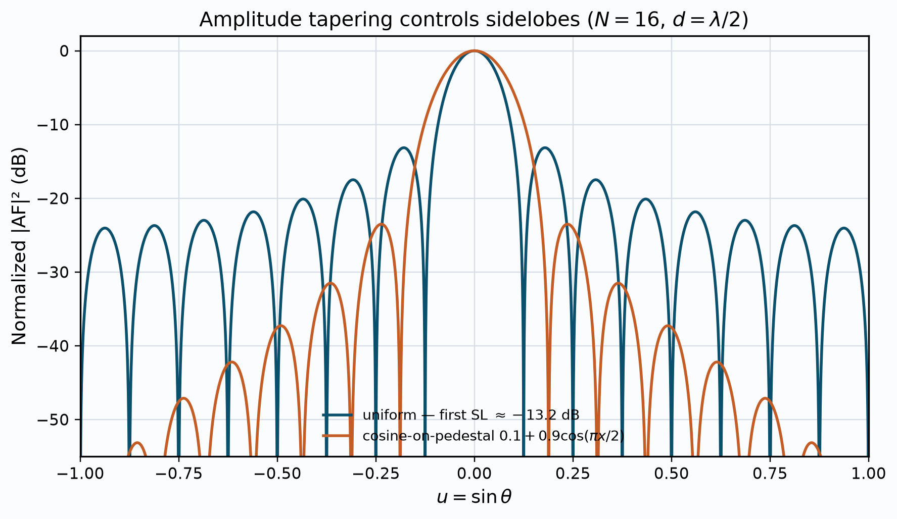
Two questions come up all the time. First: if my element already has nulls, what happens to the array pattern? Second: uniform weights give first sidelobes near \(-13\,\mathrm{dB}\)—how do I buy lower sidelobes? We answer both with formulas you can run.
Technical development
\[G_{\mathrm{total}}(\theta,\phi)\propto G_{\mathrm{element}}(\theta,\phi)\,\bigl|A(\theta,\phi)\bigr|^2.\]For tapering, replace uniform weights by a window \(w_n\) (cosine-on-pedestal, Taylor, Chebyshev, and so on). Lower edge illumination lowers near sidelobes, widens the main beam, and reduces aperture efficiency.
How this achieves the motive
In Figure 1 the element nulls cut into the product even where the array factor is strong. In Figure 2 you see the sidelobe cost of uniform illumination and the beamwidth cost of tapering. That is the usual design trade.
Sample simulation
import numpy as np
import matplotlib.pyplot as plt

def array_factor(u, N, d_over_lambda, u0=0.0, weights=None):
    """Normalized |AF(u)|^2, u=sin(theta)."""
    if weights is None:
        weights = np.ones(N)
    weights = np.asarray(weights, dtype=float)
    weights = weights / np.max(np.abs(weights))
    kdl = 2 * np.pi * d_over_lambda
    af = np.zeros_like(u, dtype=complex)
    for n in range(N):
        af += weights[n] * np.exp(1j * n * kdl * (u - u0))
    g = np.abs(af) ** 2
    return g / np.max(g)

def db(g, floor=-60.0):
    return 10 * np.log10(np.maximum(g, 10 ** (floor / 10)))

phi = np.linspace(0, 2*np.pi, 1441)
N, d = 8, 0.5
kdl = 2*np.pi*d
AF = np.zeros_like(phi, dtype=complex)
for n in range(N):
    AF += np.exp(1j * n * kdl * np.cos(phi))
G_af = np.abs(AF)**2; G_af /= np.max(G_af)
G_el = np.maximum(np.cos(phi)**2, 0); G_el /= np.max(G_el)
G_tot = G_af*G_el; G_tot /= np.max(G_tot)
fig, axes = plt.subplots(1, 3, subplot_kw=dict(projection="polar"), figsize=(12, 4))
for ax, g, title in zip(axes, [G_el, G_af, G_tot], ["Element", "AF", "Product"]):
    ax.plot(phi, g); ax.set_ylim(0, 1.08); ax.set_title(title)
plt.show()
u = np.linspace(-1, 1, 4001)
N, d = 16, 0.5
n = np.arange(N)
x = (n - (N-1)/2)/((N-1)/2)
w_uni = np.ones(N)
w_cos = 0.1 + 0.9*np.cos(0.5*np.pi*x)
plt.plot(u, db(array_factor(u, N, d, weights=w_uni)), label="uniform")
plt.plot(u, db(array_factor(u, N, d, weights=w_cos)), label="cosine-on-pedestal")
plt.xlabel("u"); plt.ylabel("dB"); plt.ylim(-55, 2); plt.grid(True); plt.legend(); plt.show()
Sample results
The three-panel polar plot should match Figure 1. The taper plot should match Figure 2: first sidelobes drop well below \(-13\,\mathrm{dB}\), and the main beam widens.
Next topic
That is the set of four design levers for a ULA: spacing sets aliasing, progressive phase steers, taper controls sidelobes, and the element pattern multiplies the array factor. Mutual coupling, digital beamforming, and calibration sit on top of the same structure.
References
[1] Balanis. [2] Mailloux. [3] Orfanidis.