Key focus: Learn how to generate color noise using auto regressive (AR) model. Apply Yule Walker equations for generating power law noises: pink noise, Brownian noise.
Auto-Regressive (AR) model
An uncorrelated Gaussian random sequence can be transformed into a correlated Gaussian random sequence using an AR time-series model. If a time series random sequence is assumed to be following an auto-regressive model of form,
where is the uncorrelated Gaussian sequence of zero mean and variance , the natural tendency is to estimate the model parameters . Least Squares method can be applied here to find the model parameters, but the computations become cumbersome as the order increases. Fortunately, the AR model coefficients can be solved for using Yule Walker equations.
Yule Walker equations relate auto-regressive model parameters to the auto-correlation of random process . Finding the model parameters using Yule-Walker equations, is a two step process:
1. Given , estimate auto-correlation of the process . If is already specified as a function, utilize it as it is (see auto-correlation equations for Jakes spectrum or Doppler spectrum in section 11.3.2 in the book).
2. Solve Yule Walker equations to find the model parameters and the noise sigma .
Yule-Walker equations
Yule-Walker equations can be compactly written as
Equation (2) Yule Walker equation
Written in matrix form, the Yule-Walker equations that comprises of a set of linear equations and unknown parameters.
Representing equation (3) in a compact form,
The AR model parameters can be found by solving
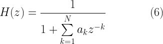
After solving for the model parameters , the noise variance can be found by applying the estimated values of in equation (2) by setting . The aryule command (in Matlab and Python’s spectrum package) efficiently solves the Yule-Walker equations using Levinson Algorithm [1][2]. Once the model parameters are obtained, the AR model can be implemented as an \emph{infinte impulse response (IIR)} filter of form
Example: power law noise generation
The power law in the power spectrum characterizes the fluctuating observables in many natural systems. Many natural systems exhibit some noise which is a stochastic process with a power spectral density having a power exponent that can take values . Simply put, noise is a colored noise with a power spectral density of over its entire frequency range.
The noise can be classified into different types based on the value of .
Violet noise – = -2, the power spectral density is proportional to . Blue noise – = -1, the power spectral density is proportional to . White noise – = 0, the power spectral density is flat across the whole spectrum. Pink noise – = 1, the power spectral density is proportional to , i.e, it decreases by per octave with increase in frequency. Brownian noise – = 2, the power spectral density is proportional to , therefore it decreases by per octave with increase in frequency.
The power law noise can be generated by sequencing a zero-mean white noise through an auto-regressive (AR) filter of order :
where, is a zero-mean white noise process. Referring the AR generation method described in [3], the coefficients of the AR filter can be generated as
which can be implemented as an infinite impulse response (IIR) filter using the filter transfer function described in equation (6).
The following script implements this method and the sample results are plotted in the next Figure.
The aim of this article is to demonstrate the application of spectral factorization method in generating colored noise having Jakes power spectral density. Before continuing, I urge the reader to go through this post: Introduction to generating correlated Gaussian sequences.
In spectral factorization method, a filter is designed using the desired frequency domain characteristics (like PSD) to transform an uncorrelated Gaussian sequence into a correlated sequence . In the model shown in Figure 1, the input to the LTI system is a white noise whose amplitude follows Gaussian distribution with zero mean and variance and the power spectral density (PSD) of the white noise is a constant across all frequencies.
The white noise sequence drives the LTI system with frequency response producing the signal of interest . The PSD of the output process is therefore
Figure 1: Relationship among various power spectral densities in a filtering process
If the desired power spectral density of the colored noise sequence is given, assuming , the impulse response of the LTI filter can be found by taking the inverse Fourier transform of the frequency response
Once, the impulse response of the filter is obtained, the colored noise sequence can be produced by driving the filter with a zero-mean white noise sequence of unit variance.
Example: Generating colored noise with Jakes PSD
For example, we wish to generate a Gaussian noise sequence whose power spectral density follows the normalized Jakes power spectral density (see section 11.3.2 in the book) given by
Applying spectral factorization method, the frequency response of the desired filter is
The impulse response of the filter is [1]
where, is the fractional Bessel function of the first kind, is the sampling interval for implementing the digital filter and is a constant. The impulse response of the filter can be normalized by dividing by .
The filter can be implemented as a finite impulse response (FIR) filter structure. However, the FIR implementation requires that the impulse response be truncated to a reasonable length. Such truncation leads to ringing effects due to Gibbs phenomenon. To avoid distortions due to truncation, the filter impulse response is usually windowed using a window function such as Hamming window.
where, the Hamming window is defined as
The function given in the book in section 2.6.1 implements a windowed Jakes filterusing the aforementioned equations. The impulse response and the spectral characteristics of the filter are plotted in Figure 2.
Figure 2: Impulse response & spectrum of windowed Jakes filter ( fmax = 10Hz; Ts = 0:01s; N = 512)
A white noise can be transformed into colored noise sequence with Jakes PSD, by processing the white noise through the implemented filter. The script (given in the book in section 2.6.1) illustrates this concept by transforming a white noise sequence into a colored noise sequence. The simulated noise samples and its PSD are plotted in Figure 3.
Key focus: Colored noise sequence (a.k.a correlated Gaussian sequence), is a non-white random sequence, with non-constant power spectral density across frequencies.
Introduction
Speaking of Gaussian random sequences such as Gaussian noise, we generally think that the power spectral density (PSD) of such Gaussian sequences is flat.We should understand that the PSD of a Gausssian sequence need not be flat. This bring out the difference between white and colored random sequences, as captured in Figure 1.
A white noise sequence is defined as any random sequence whose PSD is constant across all frequencies. Gaussian white noise is a Gaussian random sequence, whose amplitude is gaussian distributed and its PSD is a constant. Viewed in another way, a constant PSD in frequency domain implies that the average auto-correlation function in time-domain is an impulse function (Dirac-delta function). That is, the amplitude of noise at any given time instant is correlated only with itself. Therefore, such sequences are also referred as uncorrelated random sequences. White Gaussian noise processes are completely characterized by its mean and variance.
Figure 1: Power spectral densities of white noise and colored noise
A colored noise sequence is simply a non-white random sequence, whose PSD varies with frequency. For a colored noise, the amplitude of noise at any given time instant is correlated with the amplitude of noise occurring at other instants of time. Hence, colored noise sequences will have an auto-correlation function other than the impulse function. Such sequences are also referred as correlated random sequences. Colored Gaussian noise processes are completely characterized by its mean and the shaped of power spectral density (or the shape of auto-correlation function).
In mobile channel model simulations, it is often required to generate correlated Gaussian random sequences with specified mean and power spectral density (like Jakes PSD or Gaussian PSD given in section 11.3.2 in the book). An uncorrelated Gaussian sequence can be transformed into a correlated sequence through filtering or linear transformation, that preserves the Gaussian distribution property of amplitudes, but alters only the correlation property (equivalently the power spectral density). We shall see two methods to generate colored Gaussian noise for given mean and PSD shape
Let’s say we observe a real world signal that has an arbitrary spectrum . We would like to describe the long sequence of using very few parameters, as in applications like linear predictive coding (LPC). The modeling approach, described here, tries to answer the following two questions:
• Is it possible to model the first order (mean/variance) and second order (correlations, spectrum) statistics of the signal just by shaping a white noise spectrum using a transfer function ? (see Figure 1). • Does this produce the same statistics (spectrum, correlations, mean and variance) for a white noise input ?
If the answer is yes to the above two questions, we can simply set the modeled parameters of the system and excite the system with white noise, to produce the desired real world signal. This reduces the amount to data we wish to transmit in a communication system application. This approach can be used to transform an uncorrelated white Gaussian noise sequence to a colored Gaussian noise sequence with desired spectral properties.
A random process (or signal for your visualization) with a constant power spectral density (PSD) function is a white noise process.
Power Spectral Density
Power Spectral Density function (PSD) shows how much power is contained in each of the spectral component. For example, for a sine wave of fixed frequency, the PSD plot will contain only one spectral component present at the given frequency. PSD is an even function and so the frequency components will be mirrored across the Y-axis when plotted. Thus for a sine wave of fixed frequency, the double sided plot of PSD will have two components – one at +ve frequency and another at –ve frequency of the sine wave. (Know how to plot PSD/FFT in Python & in Matlab)
Gaussian and Uniform White Noise:
A white noise signal (process) is constituted by a set of independent and identically distributed (i.i.d) random variables. In discrete sense, the white noise signal constitutes a series of samples that are independent and generated from the same probability distribution. For example, you can generate a white noise signal using a random number generator in which all the samples follow a given Gaussian distribution. This is called White Gaussian Noise (WGN) or Gaussian White Noise. Similarly, a white noise signal generated from a Uniform distribution is called Uniform White Noise.
Gaussian Noise and Uniform Noise are frequently used in system modelling. In modelling/simulation, white noise can be generated using an appropriate random generator. White Gaussian Noise can be generated using randn function in Matlab which generates random numbers that follow a Gaussian distribution. Similarly, rand function can be used to generate Uniform White Noise in Matlab that follows a uniform distribution. When the random number generators are used, it generates a series of random numbers from the given distribution. Let’s take the example of generating a White Gaussian Noise of length 10 using randn function in Matlab – with zero mean and standard deviation=1.
This simply generates 10 random numbers from the standard normal distribution. As we know that a white process is seen as a random process composing several random variables following the same Probability Distribution Function (PDF). The 10 random numbers above are generated from the same PDF (standard normal distribution). This condition is called “identically distributed” condition. The individual samples given above are “independent” of each other. Furthermore, each sample can be viewed as a realization of one random variable. In effect, we have generated a random process that is composed of realizations of 10 random variables. Thus, the process above is constituted from “independent identically distributed” (i.i.d) random variables.
Strictly and weakly defined white noise:
Since the white noise process is constructed from i.i.d random variable/samples, all the samples follow the same underlying probability distribution function (PDF). Thus, the Joint Probability Distribution function of the process will not change with any shift in time. This is called a stationary process. Hence, this noise is a stationary process. As with a stationary process which can be classified as Strict Sense Stationary (SSS) and Wide Sense Stationary (WSS) processes, we can have white noise that is SSS and white noise that is WSS. Correspondingly they can be called strictly defined white noise signal and weakly defined white noise signal.
What’s with Covariance Function/Matrix ?
A white noise signal, denoted by \(x(t)\), is defined in weak sense is a more practical condition. Here, the samples are statistically uncorrelated and identically distributed with some variance equal to \(\sigma^2\). This condition is specified by using a covariance function as
\[COV \left(x_i, x_j \right) = \begin{cases} \sigma^2, & \quad i = j \\ 0, & \quad i \neq j \end{cases}\]
Why do we need a covariance function? Because, we are dealing with a random process that is composed of \(n\) random variables (10 variables in the modelling example above). Such a process is viewed as multivariate random vector or multivariate random variable.
For multivariate random variables, Covariance function specified how each of the \(n\) variables in the given random process behaves with respect to each other. Covariance function generalizes the notion of variance to multiple dimensions.
The above equation when represented in the matrix form gives the covariance matrix of the white noise random process. Since the random variables in this process are statistically uncorrelated, the covariance function contains values only along the diagonal.
The matrix above indicates that only the auto-correlation function exists for each random variable. The cross-correlation values are zero (samples/variables are statistically uncorrelated with respect to each other). The diagonal elements are equal to the variance and all other elements in the matrix are zero.The ensemble auto-correlation function of the weakly defined white noise is given by This indicates that the auto-correlation function of weakly defined white noise process is zero everywhere except at lag \(\tau=0\).
\[R_{xx}(\tau) = E \left[ x(t) x^*(t-\tau)\right] = \sigma^2 \delta (\tau)\]
Wiener-Khintchine Theorem states that for Wide Sense Stationary Process (WSS), the power spectral density function \(S_{xx}(f)\) of a random process can be obtained by Fourier Transform of auto-correlation function of the random process. In continuous time domain, this is represented as
\[S_{xx}(f) = F \left[R_{xx}(\tau) \right] = \int_{-\infty}^{\infty} R_{xx} (\tau) e ^{- j 2 \pi f \tau} d \tau\]
For the weakly defined white noise process, we find that the mean is a constant and its covariance does not vary with respect to time. This is a sufficient condition for a WSS process. Thus we can apply Weiner-Khintchine Theorem. Therefore, the power spectral density of the weakly defined white noise process is constant (flat) across the entire frequency spectrum (Figure 1). The value of the constant is equal to the variance or power of the noise signal.
\[S_{xx}(f) = F \left[R_{xx}(\tau) \right] = \int_{-\infty}^{\infty} \sigma^2 \delta (\tau) e ^{- j 2 \pi f \tau} d \tau = \sigma^2 \int_{-\infty}^{\infty} \delta (\tau) e ^{- j 2 \pi f \tau} = \sigma^2\]
Figure 1: Weiner-Khintchine theorem illustrated
Testing the characteristics of White Gaussian Noise in Matlab:
Generate a Gaussian white noise signal of length \(L=100,000\) using the randn function in Matlab and plot it. Let’s assume that the pdf is a Gaussian pdf with mean \(\mu=0\) and standard deviation \(\sigma=2\). Thus the variance of the Gaussian pdf is \(\sigma^2=4\). The theoretical PDF of Gaussian random variable is given by
subplot(2,1,2)
n=100; %number of Histrogram bins
[f,x]=hist(X,n);
bar(x,f/trapz(x,f)); hold on;
%Theoretical PDF of Gaussian Random Variable
g=(1/(sqrt(2*pi)*sigma))*exp(-((x-mu).^2)/(2*sigma^2));
plot(x,g);hold off; grid on;
title('Theoretical PDF and Simulated Histogram of White Gaussian Noise');
legend('Histogram','Theoretical PDF');
xlabel('Bins');
ylabel('PDF f_x(x)');
Figure 3: Plot of simulated & theoretical PDF for Gaussian RV
Compute the auto-correlation function of the white noise. The computed auto-correlation function has to be scaled properly. If the ‘xcorr’ function (inbuilt in Matlab) is used for computing the auto-correlation function, use the ‘biased’ argument in the function to scale it properly.
figure();
Rxx=1/L*conv(flipud(X),X);
lags=(-L+1):1:(L-1);

%Alternative method
%[Rxx,lags] =xcorr(X,'biased');
%The argument 'biased' is used for proper scaling by 1/L
%Normalize auto-correlation with sample length for proper scaling

plot(lags,Rxx);
title('Auto-correlation Function of white noise');
xlabel('Lags')
ylabel('Correlation')
grid on;
Figure 4: Autocorrelation function of generated noise
Simulating the PSD:
Simulating the Power Spectral Density (PSD) of the white noise is a little tricky business. There are two issues here 1) The generated samples are of finite length. This is synonymous to applying truncating an infinite series of random samples. This implies that the lags are defined over a fixed range. ( FFT and spectral leakage – an additional resource on this topic can be found here) 2) The random number generators used in simulations are pseudo-random generators. Due these two reasons, you will not get a flat spectrum of psd when you apply Fourier Transform over the generated auto-correlation values.The wavering effect of the psd can be minimized by generating sufficiently long random signal and averaging the psd over several realizations of the random signal.
Simulating Gaussian White Noise as a Multivariate Gaussian Random Vector:
To verify the power spectral density of the white noise, we will use the approach of envisaging the noise as a composite of \(N\) Gaussian random variables. We want to average the PSD over \(L\) such realizations. Since there are \(N\) Gaussian random variables (\(N\) individual samples) per realization, the covariance matrix \( C_{xx}\) will be of dimension \(N \times N\). The vector of mean for this multivariate case will be of dimension \(1 \times N\).
Cholesky decomposition of covariance matrix gives the equivalent standard deviation for the multivariate case. Cholesky decomposition can be viewed as square root operation. Matlab’s randn function is used here to generate the multi-dimensional Gaussian random process with the given mean matrix and covariance matrix.
%Verifying the constant PSD of White Gaussian Noise Process
%with arbitrary mean and standard deviation sigma

mu=0; %Mean of each realization of Noise Process
sigma=2; %Sigma of each realization of Noise Process

L = 1000; %Number of Random Signal realizations to average
N = 1024; %Sample length for each realization set as power of 2 for FFT

%Generating the Random Process - White Gaussian Noise process
MU=mu*ones(1,N); %Vector of mean for all realizations
Cxx=(sigma^2)*diag(ones(N,1)); %Covariance Matrix for the Random Process
R = chol(Cxx); %Cholesky of Covariance Matrix
%Generating a Multivariate Gaussian Distribution with given mean vector and
%Covariance Matrix Cxx
z = repmat(MU,L,1) + randn(L,N)*R;
Compute PSD of the above generated multi-dimensional process and average it to get a smooth plot.
%By default, FFT is done across each column - Normal command fft(z)
%Finding the FFT of the Multivariate Distribution across each row
%Command - fft(z,[],2)
Z = 1/sqrt(N)*fft(z,[],2); %Scaling by sqrt(N);
Pzavg = mean(Z.*conj(Z));%Computing the mean power from fft

normFreq=[-N/2:N/2-1]/N;
Pzavg=fftshift(Pzavg); %Shift zero-frequency component to center of spectrum
plot(normFreq,10*log10(Pzavg),'r');
axis([-0.5 0.5 0 10]); grid on;
ylabel('Power Spectral Density (dB/Hz)');
xlabel('Normalized Frequency');
title('Power spectral density of white noise');
Figure 5: Power spectral density of generated noise
The PSD plot of the generated noise shows almost fixed power in all the frequencies. In other words, for a white noise signal, the PSD is constant (flat) across all the frequencies (\(- \infty\) to \(+\infty\)). The y-axis in the above plot is expressed in dB/Hz unit. We can see from the plot that the \(constant \; power = 10 log_{10}(\sigma^2) = 10 log_{10}(4) = 6\; dB\).
Application
In channel modeling, we often come across additive white Gaussian noise (AWGN) channel. To know more about the channel model and its simulation, continue reading this article: Simulate AWGN channel in Matlab & Python.
Rate this article: Note: There is a rating embedded within this post, please visit this post to rate it.
This website uses cookies to improve your experience while you navigate through the website. Out of these, the cookies that are categorized as necessary are stored on your browser as they are essential for the working of basic functionalities of the website. We also use third-party cookies that help us analyze and understand how you use this website. These cookies will be stored in your browser only with your consent. You also have the option to opt-out of these cookies. But opting out of some of these cookies may affect your browsing experience.
Necessary cookies are absolutely essential for the website to function properly. These cookies ensure basic functionalities and security features of the website, anonymously.
Cookie
Duration
Description
cookielawinfo-checbox-analytics
11 months
This cookie is set by GDPR Cookie Consent plugin. The cookie is used to store the user consent for the cookies in the category "Analytics".
cookielawinfo-checbox-analytics
11 months
This cookie is set by GDPR Cookie Consent plugin. The cookie is used to store the user consent for the cookies in the category "Analytics".
cookielawinfo-checbox-functional
11 months
The cookie is set by GDPR cookie consent to record the user consent for the cookies in the category "Functional".
cookielawinfo-checbox-functional
11 months
The cookie is set by GDPR cookie consent to record the user consent for the cookies in the category "Functional".
cookielawinfo-checbox-others
11 months
This cookie is set by GDPR Cookie Consent plugin. The cookie is used to store the user consent for the cookies in the category "Other.
cookielawinfo-checbox-others
11 months
This cookie is set by GDPR Cookie Consent plugin. The cookie is used to store the user consent for the cookies in the category "Other.
cookielawinfo-checkbox-necessary
11 months
This cookie is set by GDPR Cookie Consent plugin. The cookies is used to store the user consent for the cookies in the category "Necessary".
cookielawinfo-checkbox-performance
11 months
This cookie is set by GDPR Cookie Consent plugin. The cookie is used to store the user consent for the cookies in the category "Performance".
viewed_cookie_policy
11 months
The cookie is set by the GDPR Cookie Consent plugin and is used to store whether or not user has consented to the use of cookies. It does not store any personal data.
Functional cookies help to perform certain functionalities like sharing the content of the website on social media platforms, collect feedbacks, and other third-party features.
Performance cookies are used to understand and analyze the key performance indexes of the website which helps in delivering a better user experience for the visitors.
Analytical cookies are used to understand how visitors interact with the website. These cookies help provide information on metrics the number of visitors, bounce rate, traffic source, etc.

![x[n]](https://s0.wp.com/latex.php?latex=x%5Bn%5D&bg=ffffff&fg=000&s=0&c=20201002)

![y[n]](https://s0.wp.com/latex.php?latex=y%5Bn%5D&bg=ffffff&fg=000&s=0&c=20201002)


![R_{yy}[k]](https://s0.wp.com/latex.php?latex=R_%7Byy%7D%5Bk%5D&bg=ffffff&fg=000&s=0&c=20201002)

![R_{yy}[n]](https://s0.wp.com/latex.php?latex=R_%7Byy%7D%5Bn%5D&bg=ffffff&fg=000&s=0&c=20201002)


![\sum_{k=0}^{k=N} a_k y[n - k] = x[n] \quad \quad \quad \quad (8)](https://s0.wp.com/latex.php?latex=%5Csum_%7Bk%3D0%7D%5E%7Bk%3DN%7D+a_k+y%5Bn+-+k%5D+%3D+x%5Bn%5D+%5Cquad+%5Cquad+%5Cquad+%5Cquad+%288%29+&bg=ffffff&fg=000&s=2&c=20201002)


![h[n]](https://s0.wp.com/latex.php?latex=h%5Bn%5D&bg=ffffff&fg=000&s=0&c=20201002)


![H(f) = \sqrt{S_{yy}(f)} = \sqrt{\pi f_{max}} \left[1- \left(f/f_{max}\right)^2\right]^{-1/4} \quad (5)](https://s0.wp.com/latex.php?latex=H%28f%29+%3D+%5Csqrt%7BS_%7Byy%7D%28f%29%7D+%3D+%5Csqrt%7B%5Cpi+f_%7Bmax%7D%7D+%5Cleft%5B1-+%5Cleft%28f%2Ff_%7Bmax%7D%5Cright%29%5E2%5Cright%5D%5E%7B-1%2F4%7D+%5Cquad+%285%29+&bg=ffffff&fg=000&s=2&c=20201002)

![h[n] = C f_{max} x^{-1/4} J_{1/4} (x) , \quad \quad x = 2 \pi f_{max} |n T_s| \quad (6)](https://s0.wp.com/latex.php?latex=h%5Bn%5D+%3D+C+f_%7Bmax%7D+x%5E%7B-1%2F4%7D+J_%7B1%2F4%7D+%28x%29+%2C+%5Cquad+%5Cquad+x+%3D+2+%5Cpi+f_%7Bmax%7D+%7Cn+T_s%7C+%5Cquad+%286%29+&bg=ffffff&fg=000&s=2&c=20201002)


![h_{norm}[n] = x^{-1/4} J_{1/4} (x), \quad \quad x = 2 \pi f_{max} |n T_s| \quad (7)](https://s0.wp.com/latex.php?latex=h_%7Bnorm%7D%5Bn%5D+%3D+x%5E%7B-1%2F4%7D+J_%7B1%2F4%7D+%28x%29%2C+%5Cquad+%5Cquad+x+%3D+2+%5Cpi+f_%7Bmax%7D+%7Cn+T_s%7C+%5Cquad+%287%29+&bg=ffffff&fg=000&s=2&c=20201002)

![h_{w}[n] = h_{norm}[n] w_{H}[n] \quad \quad (8)](https://s0.wp.com/latex.php?latex=h_%7Bw%7D%5Bn%5D+%3D+h_%7Bnorm%7D%5Bn%5D+w_%7BH%7D%5Bn%5D+%5Cquad+%5Cquad+%288%29+&bg=ffffff&fg=000&s=2&c=20201002)

![w_{H}[n] = 0.54-0.46 \; cos(2 \pi n /N) \quad \quad (9)](https://s0.wp.com/latex.php?latex=w_%7BH%7D%5Bn%5D+%3D+0.54-0.46+%5C%3B+cos%282+%5Cpi+n+%2FN%29+%5Cquad+%5Cquad+%289%29+&bg=ffffff&fg=000&s=2&c=20201002)


