Young’s model for Rayleigh fading — filtered Gaussian discrete-time simulation

Fading & Diversity — 6 lessons (same on every page in this path)

1. Rayleigh BER → 2. Clarke’s model → 3. Young’s model (you are here) → 4. SIMO models → 5. Selection combining → 6. MRC

Tools: BER vs Eb/N0 · 3GPP TDL · CDL / Doppler

Lesson 3 of 6. Another standard way to generate Rayleigh processes after Clarke. Next we add antennas: SIMO / receive-diversity channel models.

Introduction

Young and Beaulieu’s construction is a way to generate a time series of correlated Rayleigh fades with the classical Jakes (Clarke) Doppler spectrum. It is a modification of Smith’s inverse-DFT method. It is not, by itself, a frequency-selective channel. Frequency selectivity needs a tapped delay line, with one such process on each tap. What this article builds is the complex coefficient of a flat fading channel, evolving in time.

The physical picture is the usual one. Many paths arrive with different delays and angles, none of them a dominant line of sight, so the baseband coefficient is a zero-mean complex Gaussian and its amplitude is Rayleigh. Motion between the transmitter and the receiver spreads that coefficient in frequency. The spectrum used here is the U-shaped Jakes spectrum, band-limited to the maximum Doppler frequency \(f_d\).

Young’s model

In the previous article, the characteristics and types of fading was discussed. Rayleigh Fading channel with Doppler shift is considered in this article.

Consider a channel affected by both Rayleigh Fading phenomena and Doppler Shift. Rayleigh Fading is caused due to multipath reflections of the received signal before it reaches the receiver and the Doppler Shift is caused due to the difference in the relative velocity/motion between the transmitter and the receiver. This scenario is encountered in day to day mobile communications.

Several algorithms produce correlated Rayleigh samples. David J. Young and Norman C. Beaulieu, in “The Generation of Correlated Rayleigh Random Variates by Inverse Discrete Fourier Transform” [1], start from Smith’s IDFT method and rearrange it. Their rearrangement uses one IDFT instead of two, and about two thirds of the memory, because a single complex transform supplies both quadrature components.

Rayleigh Fading can be simulated by adding two Gaussian Random variables as mentioned in my previous post. The effect of Doppler shift is incorporated by modeling the Doppler effect as a frequency domain filter.

The model proposed by Young et.al is shown below.

Rayleigh Fading - Young's model — Rayleigh Fading – Young’s model

The Fading effect + Doppler Shift is simulated by multiplying the Gaussian Random variables and the Doppler Shift’s Frequency domain representation. Then IDFT is performed to bring them into time domain representation. The Doppler Filter used to represent the Doppler Shift effect is derived in Young’s paper.

Let \(f_m = f_d/f_s\) be the maximum Doppler frequency normalised by the sampling rate, and let \(k_m = \lfloor N f_m \rfloor\). The Doppler filter that shapes an \(N\)-point white spectrum is

\[F[k]=\begin{cases} 0, & k=0 \\[4pt] \sqrt{\dfrac{1}{2\sqrt{1-\left(\dfrac{k}{N f_m}\right)^2}}}, & k=1,2,\ldots,k_m-1 \\[6pt] \sqrt{\dfrac{k_m}{2}\left[\dfrac{\pi}{2}-\arctan\left(\dfrac{k_m-1}{\sqrt{2k_m-1}}\right)\right]}, & k=k_m \\[6pt] 0, & k=k_m+1,\ldots,N-k_m-1 \\[4pt] \sqrt{\dfrac{k_m}{2}\left[\dfrac{\pi}{2}-\arctan\left(\dfrac{k_m-1}{\sqrt{2k_m-1}}\right)\right]}, & k=N-k_m \\[6pt] \sqrt{\dfrac{1}{2\sqrt{1-\left(\dfrac{N-k}{N f_m}\right)^2}}}, & k=N-k_m+1,\ldots,N-1 \end{cases}\]

The bin at \(k = 0\) is set to zero in the paper, and the area under the singularity of the Jakes spectrum is placed in the bins \(k_m\) and \(N-k_m\). An older rendering of this equation on the page wrote a spurious backslash in front of the zero at \(k = 0\). The cases above are the filter as stated by Young and Beaulieu. \(N\) has to be large enough that \(k_m \ge 1\), otherwise the Doppler span occupies none of the DFT bins.

Python realisation

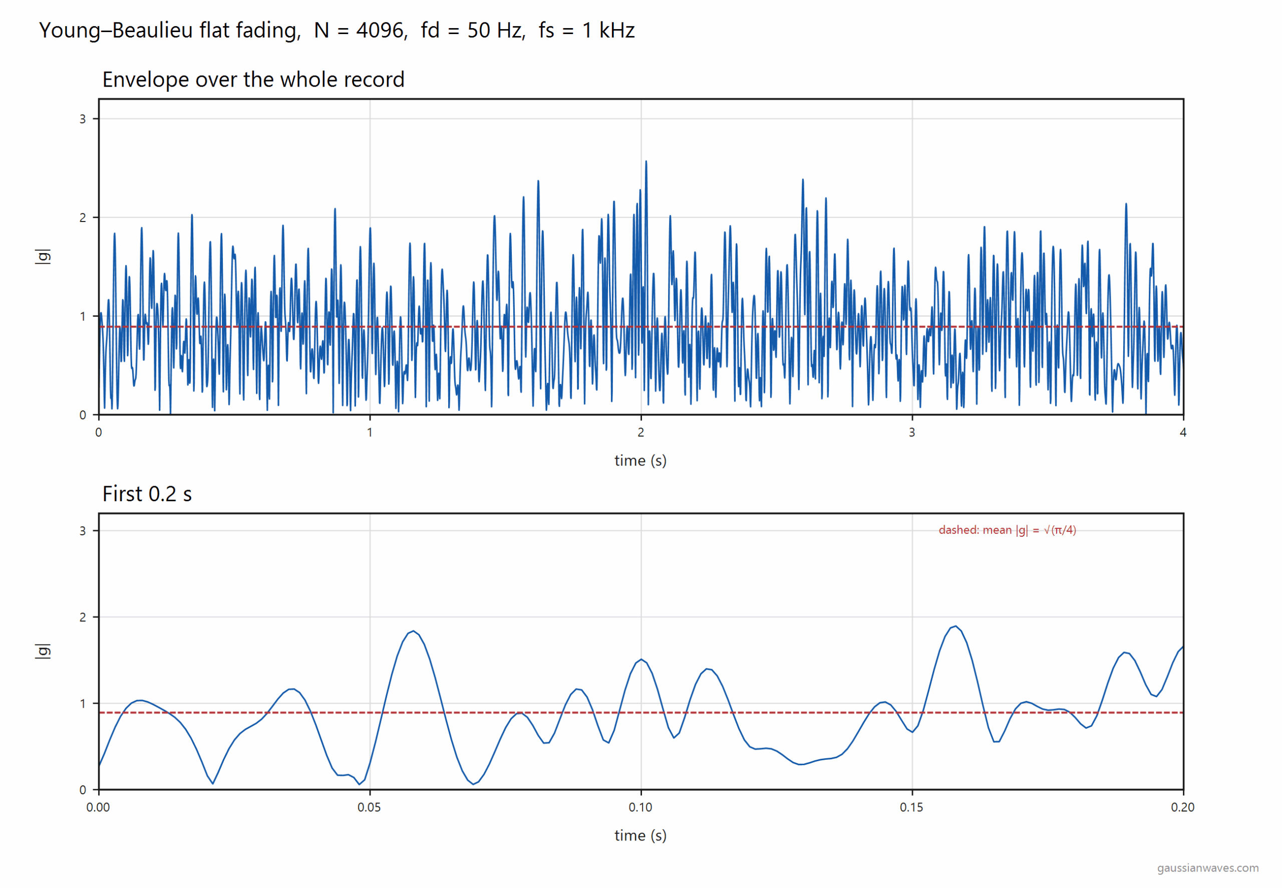
One complex IDFT produces the complex envelope. The output is scaled so that \(E[|g|^2] = 1\), which makes \(|g|\) a unit-power Rayleigh amplitude (scale \(1/\sqrt{2}\)). The example uses \(N = 4096\), \(f_d = 50\) Hz and \(f_s = 1\) kHz. The time-series plot further down is one draw at these parameters. A useful check, not done by the snippet, is to compare the measured autocorrelation against \(J_0(2\pi f_d \tau)\).

import numpy as np

def young_rayleigh(N, fd, fs, rng=None):
    """Complex flat-fading envelope with the Jakes spectrum, unit average power.

    fd and fs are in hertz. N is the DFT length. Young and Beaulieu, IEEE
    Trans. Commun., vol. 48, pp. 1114-1127, July 2000.
    """
    rng = np.random.default_rng() if rng is None else rng
    fm = fd / fs
    km = int(np.floor(fm * N))
    if km < 1:
        raise ValueError("Doppler span is empty. Increase N or fd/fs.")

    F = np.zeros(N)
    k = np.arange(1, km)
    F[k] = np.sqrt(1.0 / (2.0 * np.sqrt(1.0 - (k / (N * fm)) ** 2)))
    edge = np.sqrt((km / 2.0) * (np.pi / 2.0 - np.arctan((km - 1) / np.sqrt(2 * km - 1))))
    F[km] = edge
    F[N - km] = edge
    k2 = np.arange(N - km + 1, N)
    F[k2] = np.sqrt(1.0 / (2.0 * np.sqrt(1.0 - ((N - k2) / (N * fm)) ** 2)))

    white = (rng.normal(size=N) + 1j * rng.normal(size=N)) / np.sqrt(2.0)
    # numpy's ifft carries 1/N; multiply it back so the filter gain is F[k]
    g = np.fft.ifft(F * white) * N
    g /= np.sqrt(np.mean(np.abs(g) ** 2))
    return g

N, fd, fs = 4096, 50.0, 1000.0
g = young_rayleigh(N, fd, fs, rng=np.random.default_rng(2))
t = np.arange(N) / fs
print("samples", N, " duration %.2f s" % t[-1])
print("E[|g|^2] = %.4f,   mean amplitude = %.4f (Rayleigh theory %.4f)" % (
    np.mean(np.abs(g) ** 2), np.mean(np.abs(g)), np.sqrt(np.pi / 4.0)))

Matlab Code

Check this book for full Matlab code.
Simulation of Digital Communication Systems Using Matlab – by Mathuranathan Viswanathan

Matlab code Output:

Rayleigh envelope from the Young-Beaulieu model — *Rayleigh envelope from the listing: \(N = 4096\), \(f_d = 50\) Hz, \(f_s = 1\) kHz.*

Reference:

[1] D.J. Young and N.C. Beaulieu, “The generation of correlated Rayleigh random variates by inverse discrete fourier transform,” IEEE transactions on Communications, vol. 48, pp. 1114-1127, July 2000.

External Resources

[1]Theoretical expressions for BER under various conditions
[2] The Manchester link that used to sit here no longer resolves. For the Doppler spectrum itself, Clarke’s 1968 paper and the Young–Beaulieu paper cited above are the stable references.

Python sketch: Rayleigh envelope from complex Gaussians

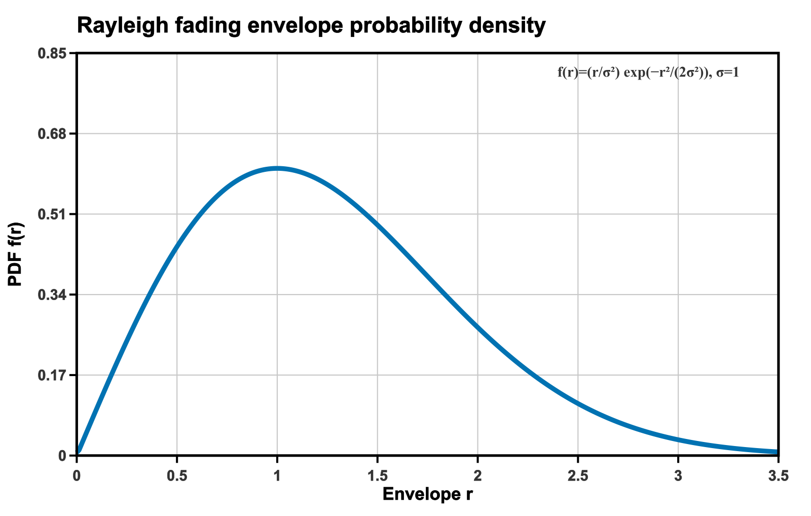
Rayleigh envelope PDF — Ideal Rayleigh PDF for the fading envelope \(r=|h|\).

Clarke’s sum-of-sinusoids builds time-correlated \(h(t)\). The marginal distribution of a well-normalized isotropic complex Gaussian still has Rayleigh envelope:

import numpy as np

N = 200_000
h = (np.random.randn(N) + 1j*np.random.randn(N)) / np.sqrt(2)  # E[|h|^2]=1
r = np.abs(h)
# crude PDF check: mean of Rayleigh(σ=1/√2) is sqrt(π/4) ≈ 0.886
print('mean envelope ~', r.mean(), ' (theory 0.886)')
print('E[|h|^2] ~', np.mean(np.abs(h)**2))

For standardized 5G delay profiles after you leave flat fading, jump to the 3GPP TDL calculator and the TDL multipath article.

← Previous: Clarke’s model Next: SIMO models →

FAQ

What is the recommended reading order? Follow the six lessons at the top: Rayleigh BER → Clarke → Young → SIMO models → Selection combining → MRC. Optional branch: Rician fading.