Understanding Gibbs Phenomenon in signal processing

Introduction

Gibbs phenomenon is a phenomenon that occurs in signal processing and Fourier analysis when approximating a discontinuous function using a series of Fourier coefficients. Specifically, it is the observation that the overshoots near the discontinuities of the approximated function do not decrease with increasing numbers of Fourier coefficients used in the approximation.

In other words, when a discontinuous function is approximated by its Fourier series, the resulting series will exhibit oscillations near the discontinuities that do not diminish as more terms are added to the series. This can lead to a “ringing” effect in the signal, where there are spurious oscillations near the discontinuity that can persist even when the number of Fourier coefficients used in the approximation is increased.

The Gibbs phenomenon is named after American physicist Josiah Willard Gibbs, who first described it in 1899. It is a fundamental limitation of the Fourier series approximation and can occur in many other areas of signal processing and analysis as well.

Gibbs phenomenon

Fourier transform represents signals in frequency domain as summation of unique combination of sinusoidal waves. Fourier transforms of various signals are shown in the Figure 1. Some of these signals, square wave and impulse, have abrupt discontinuities (sudden changes) in time domain. They also have infinite frequency content in the frequency domain.

Therefore, abrupt discontinuities in the signals require infinite frequency content in frequency domain. As we know, in order to represent these signals in computer memory, we cannot dispense infinite memory (or infinite bandwidth when capturing/measurement) to hold those infinite frequency terms. Somewhere, the number of frequency terms has to be truncated. This truncation in frequency domain manifests are ringing artifacts in time domain and vice-versa. This is called Gibbs phenomenon.

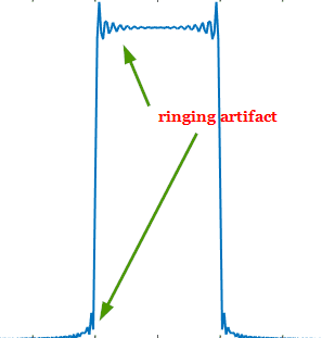
These ringing artifacts result from trying to describe the given signal with less number of frequency terms than the ideal. In practical applications, the ringing artifacts can result from

● Truncation of frequency terms – For example, to represent a perfect square wave, an infinite number of frequency terms are required. Since we cannot have an instrument with infinite bandwidth, the measurement truncates the number of frequency terms, resulting in the ringing artifact.

● Shape of filters – The ringing artifacts resulting from filtering operation is related to the sharp transitions present in the shape of the filter impulse response.

FIR filters and Gibbs phenomenon

Owing to their many favorable properties, digital Finite Impulse Response (FIR) filters are extremely popular in many signal processing applications. FIR filters can be designed to exhibit linear phase response in passband, so that the filter does not cause delay distortion (or dispersion) where different frequency components undergo different delays.

The simplest FIR design technique is the Impulse Response Truncation, where an ideal impulse response of infinite duration is truncated to finite length and the samples are delayed to make it causal. This method comes with an undesirable effect due to Gibbs Phenomenon.

Ideal brick wall characteristics in frequency domain is desired for most of the filters. For example, a typical ideal low pass filter necessitates sharp transition between passband and stopband. Any discontinuity (abrupt transitions) in one domain requires infinite number of components in the other domain.

For example, a rectangular function with abrupt transition in frequency domain translates to a \(sinc(x)=sin(x)/x\) function of infinite duration in time domain. In practical filter design, the FIR filters are of finite length. Therefore, it is not possible to represent an ideal filter with abrupt discontinuities using finite number of taps and hence the \(sinc\) function in time domain should be truncated appropriately. This truncation of an infinite duration signal in time domain leads to a phenomenon called Gibbs phenomenon in frequency domain. Since some of the samples in time domain (equivalently harmonics in frequency domain) are not used in the reconstruction, it leads to oscillations and ringing effect in the other domain. This effect is called Gibbs phenomenon.

Similar effect can also be observed in the time domain if truncation is done in the frequency domain.

This effect due to abrupt discontinuities will exists no matter how large the number of samples  is made. The situation can be improved by using a smoothly tapering windows like Blackman, Hamming , Hanning , Keiser windows etc.,

Demonstration of Gibbs Phenomenon using Matlab:

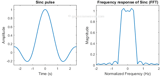
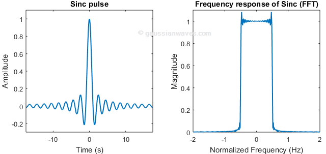
In this demonstration, a sinc pulse in time domain is considered. Sinc pulse with infinite duration in time domain, manifests as perfect rectangular shape in frequency domain. In this demo, we truncate the sinc pulse in the time domain at various length and use FFT (Fast Fourier Transform) to visualize it frequency domain. As the duration of time domain samples increases, the ringing artifact become less pronounced and the shape approaches ideal brick wall filter response.

%Gibbs Phenomenon
clearvars; % clear all stored variables

Nsyms = 5:10:60; %filter spans in symbol duration

Tsym=1; %Symbol duration
L=16; %oversampling rate, each symbol contains L samples
Fs=L/Tsym; %sampling frequency

for Nsym=Nsyms,
    [p,t]=sincFunction(L,Nsym); %Sinc Pulse

    subplot(1,2,1);
    plot(t*Tsym,p,'LineWidth',1.5);axis tight;
    ylim([-0.3,1.1]);
    title('Sinc pulse');xlabel('Time (s)');ylabel('Amplitude');
    
    [fftVals,freqVals]=freqDomainView(p,Fs,'double'); %See Chapter 1
    subplot(1,2,2);
    plot(freqVals,abs(fftVals)/abs(fftVals(length(fftVals)/2+1)),'LineWidth',1.5);
    xlim([-2 2]); ylim([0,1.1]);
    title('Frequency response of Sinc (FFT)');
    xlabel('Normalized Frequency (Hz)');ylabel('Magnitude');
    pause;% wait for user input to continue
end

Simulation Results:

I have also discussed with examples, Gibbs phenomenon applied to truncation of Fourier series coefficients. You can read about it here.

Similar articles

[1] Understanding Fourier Series
[2] Introduction to digital filter design
[3] Design FIR filter to reject unwanted frequencies
[4] FIR or IIR ? Understand the design perspective
[5] How to Interpret FFT results – complex DFT, frequency bins and FFTShift
[6] How to interpret FFT results – obtaining magnitude and phase information
[7] Analytic signal, Hilbert Transform and FFT
[8] FFT and spectral leakage
[9] Moving average filter in Python and Matlab

Books by the author

Wireless Communication Systems in Matlab Second Edition(PDF) (168 votes, average: 3.71 out of 5) $14.99 – Add to Cart Checkout Added to cart	Digital Modulations using Python (PDF ebook) (124 votes, average: 3.60 out of 5) $14.99 – Add to Cart Checkout Added to cart	Digital Modulations using Matlab (PDF ebook) (129 votes, average: 3.71 out of 5) $14.99 – Add to Cart Checkout Added to cart
Hand-picked Best books on Communication Engineering Best books on Signal Processing